Artificial Neural Network for Diagnosis
Info: 17331 words (69 pages) Dissertation
Published: 10th Dec 2019
Tagged: Biology
CHAPTER 1
INTRODUCTION
Our major concern in today’s world of 21st century fast paced lives is to maintain a good and healthy lifestyle. Due to lack of time, we tend to forget that health is the most important aspect one has to take care of and rely a lot upon others for the same. But, we have something called as Technology in our hand and when anything used in the right amount at the right time will prove to be a boon. Same goes with technology when we develop something to take care of our lifestyle and keep us away from many fatal conditions, especially diabetes, which we are going to deal with.
A person is under constant fear if he/she would be prone to any chronic disease in the near future with the present conditions he/she has. For this very purpose, a project has been designed using Artificial Neural Networks to predict the occurrence of diabetes.
Artificial Neural Network provides an excellent tool for the clinical doctors for analysis and make a sense of complicated clinical data in a wide range of medical applications. ANN applications are in the fields of medicine and generally are a classification/regression and prediction problems, i.e., that is the task basis of the measured features to give the patient to a small set of classes. ANN is a very sophisticated mathematical model widely used for diagnosis in a lot of areas like effective and efficient decision making in diagnosis and medical field, signal processing, and computer vision and so on. A doctor uses a combination of a patient’s case history and current symptoms of the disease to reach a health diagnosis when a patient is ill. In order to recognize the combination of symptoms and history that points to particular disease, the doctor’s brain accesses memory of previous patients, as well as information that has been learned from books or other doctors.
1.1 Literature Survey
Ms. Divya, Raman Chhabra, Sumit Kaur, Swagata Ghosh [1] did a detailed study on Diabetes Detection Using Artificial Neural Networks & Back-Propagation Algorithm and described the main attributes required for diabetes prediction that needs to be considered and a detailed study of the behavior of the Neural Network was studied with 200 records of data.
Scott M. Pappada, Brent D. Cameron, Paul M. Rosman[2] wrote a research paper on Development of a Neural Network for Prediction of Glucose Concentration in Type 1 Diabetes Patients which was used to study the nature of Diabetes disease.
HasanTemurtas, NejatYumusak, FeyzullahTemurtas [3] did extensive research on predicting diabetes using multi-layered neural networks and explained classification.
Jaafar [4] studied diabetes mellitus using Artificial Neural Network with the aim of determining whether someone is diabetes sufferer or not. A network of eight input layer, five hidden layers and one output layer was modeled and resultant obtained was high performance of patients diagnosed with diabetes.
Mythili, Kumar P. and Kumar R. [5] proposed a method for diagnosing diabetes mellitus based on the risk factors. Diagnosis of the same is obtained with the help Back Propagation Neural Network Algorithm in NNTool Box of MATLAB.
Jin Park and D. Edington [6] proposed and analysed sequential Neural Network Model for Diabetes Prediction
Sumanthi B. And Santha Kumaran A. [7] analysed the data of hypertension disease using the back propagation algorithm in ANN and resulted in finding out that whether patient is suffering from hypertension or not.
Meenakshi Verma [8] studied Medical Diagnosis using Back Propagation Algorithm in ANN.
After extensive research on how to proceed with working with Neural Networks, the proposed solution or method to design a Neural Network is
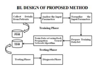
Figure 1.1 Design of Proposed Method for Medical Diagnostics using Neural Networks [8]
A. Procedure for Medical Diagnosis
(i) Data Collection and Classification – Around 800 data sets were collected from UCI repository where renowned professors and scholars share the data that they have collected from people during research. This dataset was divided into 500 records for training and 300 records for testing.
(ii) Normalizing Data –
Before giving the inputs to the network input values should be normalizedfor which we are using a built in library in Python called Scikit is used and the function “normalize” is called for the data.
B. Back Propagation (BP) Algorithm –
Backward propagating the errors is an effective neural network learning algorithm, a very common method for training artificial neural networks. To obtain a desired output, the network learns and trains itself from many inputs. The computational approach comprises of 2 parts: feed forward implementation of learned mapping and training of 3 layer network.
Algorithm for a 3 – layer network with only one hidden layer is:
- Initialize the weights in the network randomly by using random functions.
- For each record in training set O = network-output (network, e); forward pass = output e
- Calculate error at the output units in the output layer
- Compute delta(wh) for all synaptic weights from hidden layer to output layer; backward pass
- Compute delta(wi) for all weights from input layer to hidden layer; backward pass continued
- Update the weights in the network.
- As the algorithm’s name implies, the errors propagates backwards from the output nodes to the inner nodes by simultaneously updating the weights.
1.2 Introduction to Machine Learning

Figure 1.2 Machine Learning [41]
Machine learning is a part of computer sciences that gives computers the ability to learn without being programmed. Developed from the study of pattern recognition and computational learning theory in Artificial Intelligence, machine learning explores the study and building of algorithms that can all learn by itself and make almost accurate predictions on the given or obtained data. Machine learning is used in a lot of range of computing and calculating tasks where designing and programming algorithms with good efficiency is difficult or almost not feasible, the examples of its application include many new and latest applications like email filtering, detection of network intruders in a cyber-system or malicious intruders working towards a data breach, optical character recognition in understanding, learning to rank and computer vision, etc.
Figure 1.3 Machine Learning and Data Mining [42]
Machine learning is related to computational statistics, which focuses on predicting through the use of computers. It relies on mathematical techniques of optimization, theory and application domains to the field in which it is to be applied. Machine learning can be supervised or unsupervised which will be discussed further. It can be used to learn and declare baseline behavioral profiles at a very basic level for various entities and then is widely used to find similarities and meaningful anomalies.
In the field of data analytics, predictive analysis and diagnostic analysis the concepts of machine learning are used to devise and compute complex models and algorithms that lend themselves to prediction. These analytical models allow computer science researchers, data scientists, analytical engineers, and analysts to produce reliable, repeatable decisions and results and decode and deduce the hidden insights through learning from historical relationships, informative visualizations and trends in the data [9].
Supervised learning is one in which you 2 variables, an input and an output, here we have input (x) and output (Y) and an algorithm is used to learn the mapping function from the input to the output.
Y = f(X)………………………………………………(1.1)
The aim is to approximate the mapping function properly and near to perfection that when new input data (x) is entered, prediction can be made about the output variables (Y) for that data.
The algorithm continuously makes logic based predictions on the training data and is corrected. Learning of the machine halts when the algorithm achieves a required level of performance accuracy and can be resumed if not satisfied.
Regression and classification problems are few of the supervised learning algorithm branches.
- Classification: It is called classification when the output variable is a category, such as ‘true’ or ‘false’ or ‘this’ and ‘that’.
- Regression: It is called regression when the output variable is a real value, such as ‘rupees’ or ‘masses.
Some common types of problems built up on top of classification and regression modules include recommendation systems and time series prediction and analysis respectively [10].
1.2.1 Introduction to Neural Networks
Artificial neural networks (ANNs) are a mathematics based computational model which is used in computer sciences and other research disciplines, which is based on a large collection of simple units called artificial neurons, vaguely similar to the noticed behavior changes or patterns of a biological brain‘s axons.
Each neural unit is connected with many others neural units or neurons and links, which are called synapses which can improve productivity or hinder the activation state of many other adjoining neural units. Each individual neural unit computes using a function called summation function which is used to gather the input data obtained to that particular unit.
Activation function or limiting function or threshold function may be present on each connection and on that unit itself, so that the signal must cross that threshold before propagating to other neurons. These accurate systems are self-learning and trained and not explicitly programmed.
These excel in areas of solution or feature detection, which is generally difficult in traditional computers where computational capability is not as great as these analytical tools and methods.
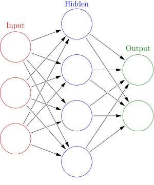
Figure 1.4 General Structure of Neural Network [43]
Neural networks usually comprise of multiple layer. The path of signal goes from first layer which is the input layer, to the last layer which is the output layer, of neural units and the middle layer with hidden units. Back Propagation uses forward stimulation to reset or change weights on the neural units and this is sometimes done in collaboration with the training where the correct result is known which is called supervised learning. More modern networks are easier and closely flowing in terms of stimulation and simulation and hesitation with connections interracting in a much more complicated, accurate and complex fashion. Dynamic or non-static neural networks are the most advanced type of neural networks, in that they newly can form new connections or disable connections and even new neural units while disabling others.
The goal of any neural network structure is to solve problems available in the way that a human brain would, though many neural networks are more impulsive in nature where not much detailing is done and intelligence should be taught. Modern neural network works work with as few as a thousand to a few million neural units and millions of neurals within, which is still several orders of magnitude less complicated than the human brain [11].
New brain research often simulates new patterns in neural networks. Other research explored with different types of signal functions over time that axons propagates, such as Deep Learning which interpolates and extends to a greater complexity than a set of boolean variables being simply on or off. This means that it can compute just more than the visible 1 and 0 values and can work on continuous values.
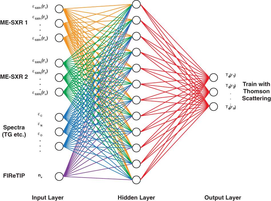
Figure 1.5 Example of Neural Network Applications, Thompson Scattering Experiment [44]
Neural networks are based on real numbers, with the value of the core typically being a value between 0.0 and 1.
An intriguing nature of these systems is that they are unpredictable and unreliable in their success with self-learning. After training, some networks become really good problem solvers and others don’t perform as well. In order to train the wonders, several thousand repetitions of interactions or epochs should occur.
Like other machine learning algorithms and methods, systems that learn from data, neural networks have been used to solve a wide variety of tasks, like computer vision and speech recognition and voice detection, that are hard to solve using ordinary rule-based programming.
Previously in the computer history, the use of neural network models marked a dramatically shift in the late 1980s from high-level (symbolic) artificial intelligence, characterized by expert systems with knowledge embodied in many conditional rules, to low-level (sub-symbolic) machine learning, characterized by knowledge embodied in the parameters of a cognitive model with some dynamical system.

Figure 1.6 Perceptron Structure [45]
There are many different types of neural networks and different models of representation, from which the multilayer perceptron is one of the most important ones. The characteristic neuron in the multilayer perceptron is the so called perceptron.
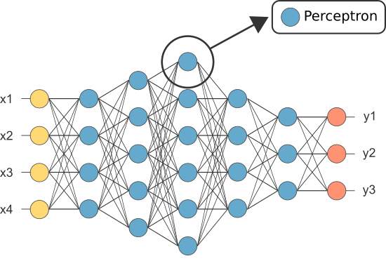
Figure 1.7 Location of Perceptron in a typical Neural Network [46]
Perceptron elements – As discussed, a neuron is the main component of a neural network, and the perceptron is the most used model. The coming figure is a graphical representation of a perceptron.
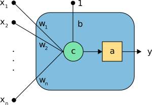
Figure 1.8 Another representation of Perceptron [46]
In the above neuron the following elements can be seen:
- The inputs (x1,…,xn).
- The bias b and the weights (w1,…,wn).
- The combination or summation function, c(·).
- The activation function a(·).
- The output y.
As an example, consider the next neuron, with three inputs. It transforms the inputs x=(x1, x2, x3) into a single output y.
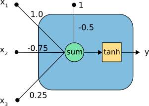
Figure 1.9 Weights on Synapses [46]
In the above neuron we can see the following elements:
- The inputs (x1, x2, x3).
- The neuron parameters, which are the set b=-0.5 and w=(1.0,-0.75,0.25).
- The combination or summation function, c(·), which merges the inputs with the bias and the weights.
- The activation function, which is set to be the hyperbolic tangent, tanh(·) or sigmoid(.), and takes that combination to produce the output from the neuron.
- The output y.
1.2.2 Types of Problems – Regression and Classification
- Classification: A classification problem is when the output variable is a category, such as “red” or “blue” or “disease” and “no disease”.
- Regression: A regression problem is called regression when the output variable is a real valued number, such as “temperature” or “weight”.
Regression is more concerned with the defining relationship between variables that are iteratively improved using an error measure in the predictions made by the model.
Regression methods are the powerhouse of working of statistics and have been adapted into statistical machine learning. This may be confusing because we can use regression to refer to the class of problem and as an algorithm. Really, regression is a process.
The most popular regression algorithms are:
- Linear Regression
- Logistic Regression
- Stepwise Regression
- Ordinary Least Squares Regression (OLSR)
- Multivariate Adaptive Regression Splines (MARS)
- Locally Estimated Scatterplot Smoothing (LOESS)
Classification is one of the Data Mining techniques that is used to analyze a given data set and takes each part of it and assigns this instance to a particular class such that error of classification will be least. It is used to extract models that accurately define important data classes within the given data set. Classification is a two-step process. During first step of prediction the model is designed by applying classification type of algorithms on training data set, then in second step the extracted model is tested against a predefined test data set to measure the model trained performance and accuracy. So classification is the process to assign class label from data set whose class label is unknown.
The most popular classification algorithms are:
- ID3 Algorithm
- Naive Bayes Algorithm
- SVM Algorithm
Diabetes prediction comes under binary classification since there are two categories, 0 (not diabetic) and 1 (diabetic) [12].
1.2.3 Attributes of Neural Networks
There are a number parameters that must be decided when designing a neural network. Among these, there are number of layers, number of neuron units per layer, the number of training iterations, etc. Some more important parameters in terms of training and network are the number of hidden neurons, the learning rate and the momentum parameter.
Number of neurons in hidden layer – Hidden neurons are the neurons that are neither in the input layer nor the output layer. These neurons are essentially hidden from seen eye, and their number and organization can typically be treated as mysterious to people who are interacting with the system. Using more hidden neurons and layers enables a greater processing power and capacity, and system flexibility. And this addition in system flexibility and processing speed has a cost, i.e., complexity of the system increases multifold. Having too many hidden neurons is going to lead to a system of equations with more equations than there are free variables available: the system is over specified, and is incapable of generalization. Alternatively, having too few hidden neurons can prevent the system from properly fitting the input data, and reduces the richness of the system.
Learning Rate – Data type is Real Domain: [0, 1] and Typical value: 0.3.
Learning Rate is the Training parameter that controls the size of weight and bias changes in learning of the training algorithm.
Momentum – Data type is Real Domain: [0, 1] and Typical value: 0.9
Momentum simply adds a fraction of the previous weight update to the current one. The momentum is used to prevent the system from converging or stopping to a local minimum or saddle point. A high momentum can also help to increase the speed of convergence of the system to a point. However, fixing the momentum too high can create a huge risk of overshooting and increasing the minimum, which can cause the system to become unstable. A momentum coefficient, if is too low cannot avoid local minimum, and can also slow down the entire training process of the system.
Training – Data type is Integer Domain: [0, 1] and Typical value: 1
Epoch – Data type: Integer Domain: [1, ∞), Typical value: 5000000
An epoch determines when training will stop once the number of iterations exceeds epochs. When training by minimum error, this represents the maximum number of iterations.
Minimum Error – Data type: Real Domain: [0, 0.5] and Typical value: 0.01
Minimum mean square error of the epoch is the square root of the sum of squared differences between the network targets and actual outputs divided by number of patterns (only for training by minimum error) [13].
1.2.4 Activation Functions
In mathematical computational networks, the activation function is defined by the output of the existing node given an input or set of inputs after a series of mathematical operations. A standard chip on computer circuit board can be seen as a wide digital set of many active activation functions that can be either in the on state (1) or off state (0), depending on input. This is similar to the behavioral patterns of any linear perceptron, the neural unit, in the class of neural networks. However, in the nonlinear activation function, it can be such that the networks should compute nontrivial or unconventionally highly complex problems using only a small number of nodes. In neural networks this function is also called transfer function of the neuron. In biologically taken neural networks, the activation function is usually an abstract concept representing the rate of action firing on the cell. In its simplest form, this function is binary—that is, either the neuron is firing or not.
A line of positive slope can also be used to show the increase in the firing rate that occurs as the input current increases. This activation function is a linear curve in nature, and therefore has the same problems as the binary function. In addition to this, networks constructed using this model have an unstable state of convergence because neuron inputs along favored paths tend to increase without bound, as this function cannot be normalized. All problems mentioned above can be handled by using a sigmoid activation function which can be normalized. One realistic model stays at zero until the current input current is received, at which point the firing frequency increases quickly at first, but gradually approaches an asymptote at 100% firing rate. Mathematically, this looks like phi (v_{i})=U(v_{i})tanh(v_{i})} phi (v_{i})=U(v_{i})tanh(v_{i}), where the tanh function can also be replaced by any sigmoid function. This behavior is realistically reflected in the neuron because they cannot physically activate faster than a certain learning rate. This model runs into problems, however, in computational networks as it is not differentiable, a requirement in order to calculate back-propagation. The final model, then, that is used in multilayer perceptrons is a sigmoidal activation function in the form of a tanh activation function. There are two forms of this function which are commonly used: phi (v_{i})=tanh(v_{i})} phi (v_{i})=tanh(v_{i}) whose range is normalized from -1 to 1, and phi (v_{i})=(1+exp(-v_{i}))^{-1}} phi (v_{i})=(1+exp(-v_{i}))^{{-1}}.
This is vertically translated to normalize from 0 to 1. The second mentioned model is often considered more realistic biologically, but it runs into experimental and theoretical difficulties with certain types of computational fixes.
Sigmoid function – A sigmoid function is a mathematical function having an “S” shaped curve sigmoid curve. Often, sigmoid function refers to the special case of the logistic function shown in the first figure and defined by the formula.
S = 1/(1+exp ^ (-x))……………………………(1.2)
Other examples of similar shapes include the Gompertz curve (used in modeling systems that saturate at large values of t) and the ogee curve (used in the spillway of some dams). Sigmoid functions have finite limits at negative infinity and infinity, most often going either from 0 to 1 or from −1 to 1, depending on convention. A wide variety of sigmoid functions have been used as the activation function of artificial neurons, including the logistic and hyperbolic tangent functions. Sigmoid curves are also common in statistics as cumulative distribution functions (which go from 0 to 1), such as the integrals of the logistic distribution, the normal distribution, and Student’s t probability density functions [14].
A graph of a sigmoid function and its derivative looks like:
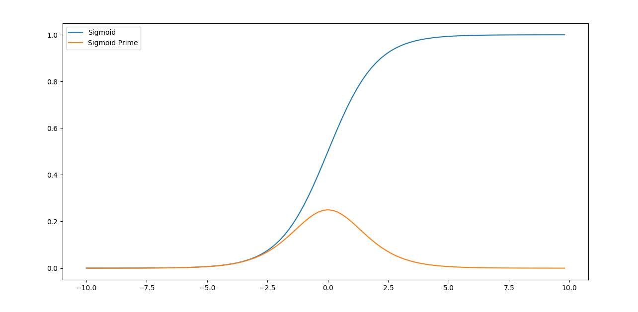
Figure 1.10 Sigmoid and Sigmoid Prime function graphs
1.2.5 Learning Algorithms
To train a neural network to make it perform some task, we should adjust the weights of each unit in such a way that the error between the expected output and the obtained output is reduced. This process requires that the neural network calculate error derivative of the weights. In other words, it must calculate how the error changes as each weight is increased or decreased either slightly or heavily. It is the easiest to understand if all the units in the network are linear. The algorithm computes each weight by first computing the function, the rate at which the error changes as the activity level of a unit is changed (at the hidden layer). For output units in the final layer, the EA is simply the difference between the actual and the desired output. To compute the function for a hidden unit in the layer only before the output layer or all the layers just before the output layer, we first identify all the weights between that hidden unit and the output units to which it is connected and then multiply those weights by the EAs of those output units and add the products. This sum equals the function for the hidden unit that is chosen. After calculating all the functions in the hidden layer just before the output layer, we can compute in like fashion the functions for other layers, moving from layer to layer in a direction opposite to the way activities propagate through the network. This is how back-propagation got its name. Once the function calculation has been computed for a unit, it is a very straight forward task to compute the weights for each incoming connection of the unit. The weights error is the product of the functions and the activity through the incoming connection. For the non-linear units, the back propagation algorithm includes an extra step of conversion into EI.
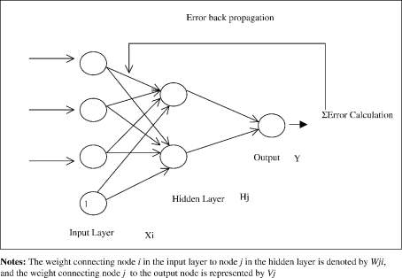
Figure 1.11 Back Propagation algorithm [47]
1.2.6 Optimization Algorithms
The procedure that is used to carry out the learning of network process in a neural network is called the training algorithm. There are many different training algorithms, with different characteristics and performance.
The learning problem in neural networks is formulated in terms of the minimization of a loss function, f. This function is in general and is composed of an error and a regularization terms. The error term evaluates how a neural network fits in the data set and learns the nature of the data. On the other hand, the regularization term is used to prevent over-fitting or under-fitting, by controlling the effective complexity of the neural network.
The loss function depends on the many changeable parameters like biases and synaptic weights in the neural network. We can group them together into an n-dimensional weight vector w. The picture below represents the loss function f(w).
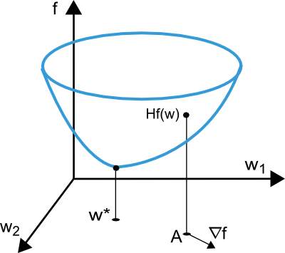
Figure 1.12 Error reduction by finding global minimum[46]
The point w* which is seen in the above context is called and is the minima of the loss function. At any point A, we can be calculate the first and second derivatives of the loss function. The very first derivatives are gropued in the famous gradient vector, whose elements can be written
ᐁif(w) = df/dwi (i = 1,…,n)…………………………..…..(1.3)
Similarly, the second derivatives of the loss function can be grouped in the Hessian matrix,
Hi,jf(w) = d2f/dwi·dwj (i,j = 1,…,n)…………………………..(1.4)
The problems of minimizing the very continuous and differentiable functions of many variables has been widely studied. Many of the traditional approaches to this problem are directly applicable to that of training neural networks.
One-dimensional optimization – Although the loss function mainly depends on many parameters, not just one, one-dimensional optimization methods are of great importance here. Indeed, they are are very often used in the training process of a neural network. And of course, many algorithms which are used for training are first compute a training direction denoted by d and then a training rate which is denoted by η that minimizes the loss in that direction, denoted by f(η).
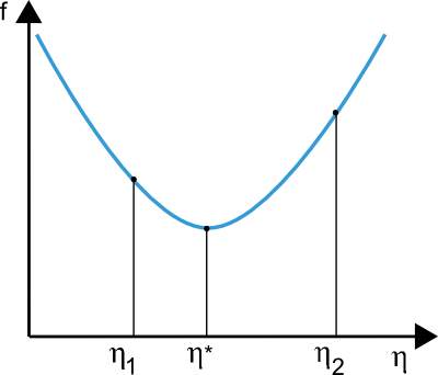
Figure 1.13 One dimensional optimization [46]
Multidimensional optimization – The learning for neural networks is developed or formulated as searching of a parameter vector w* at which the loss function f reaches a minimum value of the function. The necessary condition states that if the neural network is at a minimum of the loss function, then the gradient, difference or reduction is the zero vector. The loss function is a nonlinear function of the parameters. As a consequence, it is not possible to find closed training algorithms for the minimum value. Instead, we search through the parameter space consisting of a succeeding small steps. At each step, the loss will decrease by adjusting the parameters of neural network. In this way, to train a neural network we start with some random set of parameter vectors that is often chosen randomly. Then, we generate a sequence of parameters, so that the loss function is reduced at each iteration or epoch of the algorithm. The change of loss between two steps is called the loss decrement or gradient. The algorithm stops when a specified condition or stopping criterion is satisfied.

Figure 1.14 Five types of optimization techniques [46]
Gradient descent – Gradient descent is also known as steepest descent and is the simplest training algorithm. It requires information from the gradient vector, and hence it is a first order method.
The method begins at a point w0 and, until a stopping condition is satisfied, moves from wi to wi+1 in the training direction di = -gi. Therefore, the gradient descent method iterates in the following way:
wi+1 = wi – di·ηi, i=0,1,… ………………………………..(1.5)
The parameter η is called the training rate. This value can either be set to a fixed value or can be found out by one-dimensional optimization along the training direction at each step. An optimal value for the training rate obtained by line minimization at each successive step is that is generally preferable. Even so,there are still various software tools that use only a fixed value for the training rate. The parameter vector is improved in two steps: 1.First, the gradient descent training direction is computed and 2. suitable training rate is found after several attempts [15].
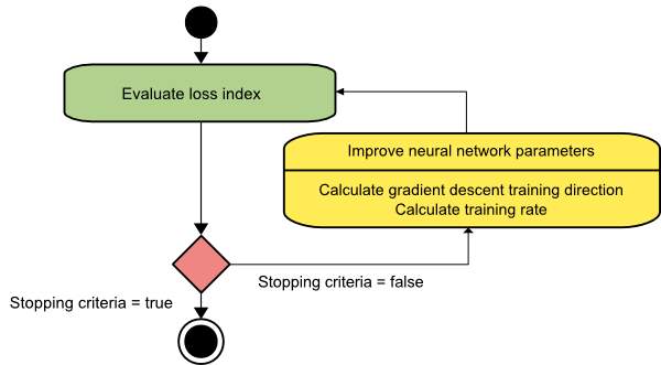
Figure 1.15 Flow-chart of Gradient Descent algorithm [46]
1.2.7 Training the Network
In training phase, the class for each record is known (this is termed supervised training), and the output nodes for the corresponding inputs can therefore be assigned “correct” values — “1” for the node corresponding to the correct class, and “0” for the others. Thus, it is possible to compare the calculated values for the output nodes to these “correct” values, and calculate an error term for each node (the “Delta” rule). These error terms are then used to adjust the weights in the hidden layers so that the next time around the output values will be closer to the “correct” values.
The Iterative Learning Process – During the iterative process, all the weights are going to get updated. Later when every case is presented, the process often starts over again. During this phase, the network learns by adjusting the weights so as to be able to predict the classification of input samples. Often Neural network learning is also referred to as connectionist learning, due to the reason that connections are present between the units. Advantages of neural networks also include their high tolerance to noisy and corrupt data, and also their ability to classify any patterns for which they have not been trained.Back-propagation algorithm is the most popular neural network algorithm there is. Once a network has been structured and designed for a particular application, that network is ready to be trained. In order to begin this process, the initial weights are chosen at random. Then the training or learning begins with some set of predefined parameters. The network processes all the records in the training data set one by one with only one at a time by using the weights and functions that are in the hidden layers. After that, it compares the resulting outputs against the desired outputs which are already known. Errors are then propagated back through the system, causing the system to adjust the weights of the network for application to the next record to be processed. This particular process occurs again and again as the weights are continuously keep on changing. During the training of neural network the same set of data is processed many times as the synapses connection weights are continually refined and redefined.
1.2.8 Testing the Network
In the testing phase, the few records that were kept aside for testing are used. This data is completely different from the original data that has been used for training. Testing mainly needs to be done to see how well our network is generalizing or captivating for all types of data which it hasn’t seen too. Generally, 3:1:1 is the ratio in which the data is divided for training, validation and testing respectively. The test outputs are compared with the expected outputs to verify the performance of the neural network. There may be cases where the training has been done extremely well but testing doesn’t turn out to be as good as training. This shows that the model is not that fit to our data as expected. All such errors are spotted during testing.
1.2.9 Problems faced by Neural Networks
The cause of poor performance in machine learning is either due to over-fitting or under-fitting of the data. In statistics, any kind of fit refers to how well we approximate the target function used for thresholding. Supervised machine learning algorithms aims to approximate the not known mapping function for the output variables based on the given input variables. Statistics often describe the goodness of fit which refers to measures used to estimate how well the approximation of the function matches the target function. Few of the methods which are useful in machine learning such as calculating the residual errors, but few techniques assume that we know the form of the target function we are approximating, which is not always the case. If we already knew the form of the target function, we would use it directly to make predictions, in place of trying to learn an approximation from samples of noisy and incomplete training data.
Over-fitting – Over-fitting refers to a model that models the training data too well. Over-fitting occurs when a model learns about the details and about the noises in the training data to that limit that it negatively impacts the performance of the model on new data which newly enters. Implying that the noise or the random fluctuations in the training data is picked up and learned as concepts by the model. Issue arising here is that these present concepts do not apply to new data and negatively impact the model’s ability to generalize. Over-fitting is more likely with non-parametric and nonlinear models that have more flexibility when learning a target function.
Under-fitting- Under-fitting refers to a model that can neither model the training data nor generalize to new data. An under-fit machine learning model is not a suitable model and will be obvious as it will have poor performance on the training data. Under-fitting is often not discussed as it is easy to detect given a good performance metric. The remedy is to move on and try alternate machine learning algorithms. Nevertheless, it does provide a good contrast to the problem of over-fitting.
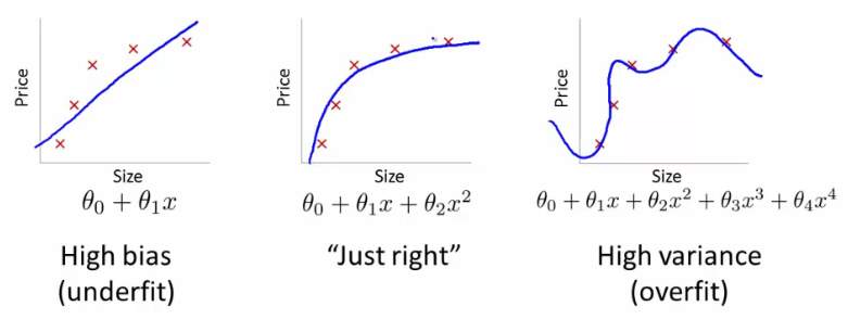
Figure 1.16 Problems faced during Training a Neural Network [48]
Good Fit – Ideally, we want to select a model at the sweet spot between under-fitting and over-fitting. This is the goal, but is very difficult to do in practice. This goal and it’s understanding requires some efforts to be put in understanding, we look at the performance of a machine learning algorithm over a period of time as it is learning a training data from the training data set. We may also plot both, the skill on the training data and the skill on a test data set we have held back from the training process. Over a period of time, as and when the algorithm learns, the error for the model on the training data decreases and so does the error on the test dataset. If we train for a very long period of time , meaning too long, the performance on the training dataset may continue to decrease as the model is over-fitting and learning the irrelevant detail and noise in the training dataset. At the same time the error for the test set starts to in again as the model’s ability to generalize decreases. The sweet spot is the point just before the error on the test dataset starts to increase where the model has good skill on both the training dataset and the unseen test dataset. [16].
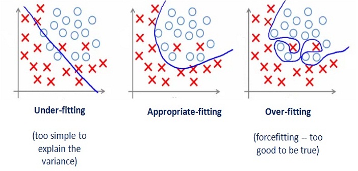
Figure 1.17 Types of fitting problems in Neural Networks [49]
CHAPTER 2
ANALYSIS
2.1 Introduction
Diseases and factors that play a major role in acquiring diabetes is described for the purpose of the analysis of this report
Diabetes represents a serious health problem in developed countries with estimated numbers reaching 366 million diabetes cases globally in 2030. It is one of metabolically acquired diseases where a patient has high blood sugar either caused by the body failure to produce enough insulin or the cells failure to respond to the produced body insulin. Diabetes can be identified or detected by studying on several readings of attributes taken from a patient such as fasting glucose, sodium, potassium, urea, creatinine, albumin and many others. Insulin is a body natural hormone which is secreted by human body by pancreas to convert sugar, starch and food to break into simpler molecules which is then used by the cells to generate energy required by daily life. Due to lack of insulin this conversion is affected and the sugar starts getting accumulated in blood stream and thus increases the blood glucose level and as a result the person develops diabetes mellitus.
Obesity (Body Fat) – Obesity is the condition whose main characteristic is the excess of fat tissue, in which the fat cells can increase in size as well as the count and results in the decrease in the quality of life and health of the individual who suffers from it. Obesity is an inherited situation and also acquired by an undisciplined conduct of eating and lifestyle. The environment has great influence over habits and attitudes that are acquired through eating. A person with inherited tendencies to be overweight can change those tendencies if he lives in a disciplined eating environment, i.e. changes his habits by a choice of his will or helpful techniques such as hypnosis or auto hypnosis. An overweight person who can change his old and deeply brought up habits and patterns of life can obtain a healthier and better life in every aspect.
Hypertension – Hypertension is a disease that affects a wide range of the population, particularly the elderly after the age of 55. It is caused by high Blood Pressure. Blood Pressure is the force of blood pushing against blood vessels walls. The heart pumps blood into the arteries (blood vessels), which carry the blood throughout the body. If blood pressure is outrageously high, there may be certain symptoms such as severe headache, fatigue, vision problems, chest pain, difficulty in breathing, irregular heartbeat and blood in the urine. Hypertension can cause stroke, heart attack, kidney failure and vision problems. Men have a greater chance of developing high Blood Pressure than women. This varies according to age and among various groups. Initial assessment of the Hypertensive affected patient should include a complete and detailed history and physical examination. [8]
2.1.1 Problem Statement
Diabetes is a chronically acquired health problem with devastating, yet preventable consequences. It is characterized by high blood glucose levels resulting from defects in insulin production, insulin action, or both. With other parameters that may affect like number of pregnancies, skin fold of a human, age, etc., design a software system that accepts user input and predicts whether the user is going to be prone to diabetes or not [17].
2.2 Software Requirement Specification (SRS)
2.2.1 Introduction
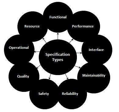
Figure 2.1 Types of SRS [50]
A software requirements specification (SRS) is a description of a software system to be developed. It lays out the required functional and non-functional requirements, and also includes a set of use cases that can describe the user interactions that the software must provide. The software requirements specification document enlists enough and necessary requirements that are required for the project development. To derive the software requirements, we should to have clear and thorough understanding of the products to be developed.
This is refined in detailed and continuous communications with the project and consumer till the completion of the software. Keeping in mind the features of an SRS document, a software system that is to be developed or that has been developed should be clearly described [18].
2.2.2 Overall Description
A software should be developed that helps the users predict whether they are prone to be diabetic or not with a few set of inputs given by them. The software works like an executable file that is platform independent and doesn’t depend on the operating system that is on the system. The software takes 8 inputs from the user namely Insulin, Age, Level of Pedigree, Number of Pregnancies, etc., and predicts the result either by 1 or 0 where 1 is diabetic and 0 being non-diabetic.
2.2.3 External Interface Requirements
External Interface Requirements include requirements like a working keyboard for a desktop system or laptop system, a screen with any resolution (User interface), a good internet connection to download the application (Communication interface) and any operating system with either of the system types (32-bit or 65-bit) (Software interface).
2.2.4 Other Non-functional Requirements
In systems engineering and requirements engineering, a non-functional requirement is a something that specifies criterion or criteria that should be used to judge the operations of a system, rather than any specific kind of behaviors without restricting the study only to a particular set of attributes that make the system work.
There are many types of non-functional requirements that can be used as the judgment parameter.
A few Non-functional requirements related to the software include:
- Accessibility – Can be accessed from any system having a fairly good internet connection.
- Dependency on other parties – doesn’t depend on any third party application to work.
- Deployment – can be deployed easily by the users themselves by downloading from the internet.
- Documentation – introductory documentation will be provided in the start of the application.
- Maintainability – easy maintenance as it doesn’t consume much space.
- Modifiability – cannot be modified by the user.
- Open source – it is not open source.
- Performance / response time (performance engineering) – 5 seconds (best case), 10 seconds (worst case)
- Platform compatibility – platform independent.
- Price – absolutely free.
- Privacy–no issues of privacy as the data will not be stored anywhere or can be hacked.
- Portability
- Readability
- Resource constraints (processor speed, memory, disk space, network bandwidth, etc.) – works faster with better processors.
- Reusability – always reusable by any number of users.
- Usability by target user community – any community of users can use.
CHAPTER 3
DESIGN
3.1 Introduction
The neural network that has been designed has a structure. It has a set of inputs and an output. The hidden layer put in the middle has perceptrons which helps in doing the internal calculations.
Layer 1 – Input Layer which is a set of records read from the system memory. Our network accepts 8 inputs as we are testing with 8 attributes taken from the dataset. The 8 inputs are:
- Number of times pregnant
- Plasma glucose concentration a 2 hours in an oral glucose tolerance test
- Diastolic blood pressure (mm Hg)
- Triceps skin fold thickness (mm)
- 2-Hour serum insulin (mu U/ml)
- Body mass index (weight in kg/(height in m)^2)
- Diabetes pedigree function
- Age (years)
Layer 2 –This layer has a set of perceptrons that do the computations and carry forward the result to the output layer. This layer consists of 10 perceptrons.
Design of the perceptron –

Figure 3.1 Design of Perceptron [46]
Layer 3 – This layer is the final output layer which is a class variable of either 1 or 0. This layer outputs a number of 1 or 0 depending on the inputs given and weights generated.
After combining all the layers, the final network looks like:
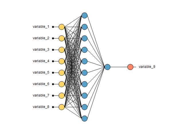
Figure 3.2 Designed Neural Network for Diabetes Prediction
Yellow color – Input layer
Blue color – Hidden layer
Red color – Output layer
3.2 UML Diagrams
UML is an authorized language for visualizing, specifying, documenting, and constructing the facts of software systems. UML stands for Unified Modeling Language. UML is a little different from the other common computer programming languages like C, Python, C++, COBOL, Java etc. UML is a pictorial representation language which is used to make software blue prints and system payouts. Therefore, UML can be described as a very general purpose visual processing language used for modelling to specify, visualize, document and construct software system. Although the concepts of UML are generally used to model and generate software systems, it is not limited within this very boundary. It is also used as a modelling concept for non-software systems like flow of process in a manufacturing unit etc.
UML is not a programming language but many tools can be used to generate code in various languages using UML diagrams. UML and OOAD are directly related. It is very important to know the difference among the various UML models. Different diagrams are used for different type of UML modeling. There are two important type of UML modelings:
Structural modeling: Structural modeling captures the static features of a system. They consist of the followings:
- Classes diagrams
- Objects diagrams
- Deployment diagrams
- Package diagrams
- Composite structure diagram
- Component diagram
Structural model represents the basic framework or distribution for the system and this framework is the place where all other components exist together. So the class diagram, component diagram and deployment diagrams are the part of structural modeling. They all are equipped with the elements, factors, tools and related mechanism to assemble them under one diagram. But the structural model can never describe the dynamism and action behavior of the system. Among all, class diagram is the most widely used structural diagram.
Behavioral Modeling: Behavioral model describes the interaction in the system. It represents the interaction among the structural diagrams. Behavioral modeling shows the dynamic nature of the system. They consist of the following:
- Activity diagrams
- Interaction diagrams
- Use case diagrams
All the above show the dynamic sequence of flow in a system [19].
Structural Modeling –We would want to present Class diagram, Object diagram, Package diagram and Component diagram.
Class diagram –
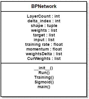
Figure 3.3 UML Diagram: Class diagram
This class has many attributes like input (list), momentum (float), etc., whose data types are also mentioned and five main functions that will be used.
Object diagram –
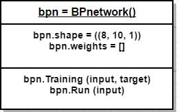
Figure 3.4 UML Diagram: Object diagram
The object used for the above class is ‘bpn’. This object accesses variables like shape and weights and functions like Training and Run.
Package diagram –
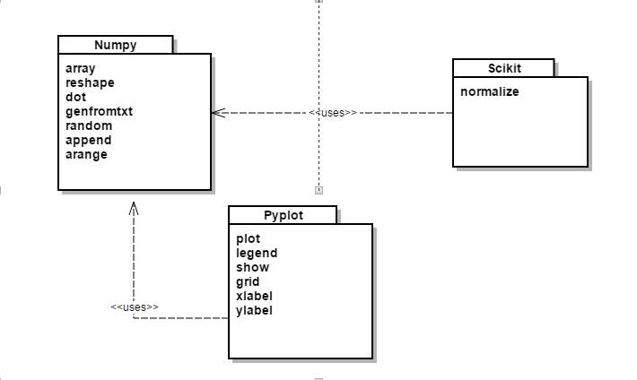
Figure 3.5 UML Diagram: Package diagram
Component diagram –
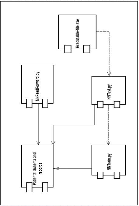
Figure 3.6 UML Diagram: Component diagram
Behavioral Modeling –We would want to present Use Case diagram, Activity diagramand State Chart diagram.
Use Case diagram – 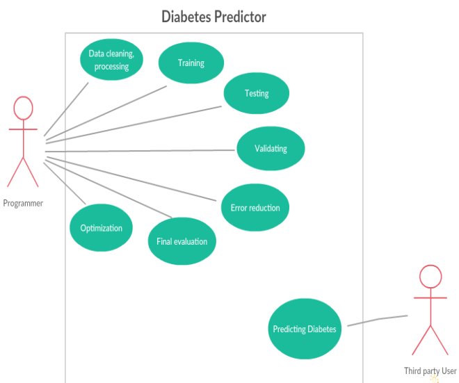
Figure 3.7 UML Diagram: Use Case diagram
This Use Case diagram shows the relationship between actors and their tasks. There are two actors here, Programmer and Third Party User. The Programmer is the one to develop the software system and train the system to generalize for all types of user data in the world. The Third Party User uses the file that has been created by the programmer by deploying it into his system and using the platform independent file.
State Chart diagram –
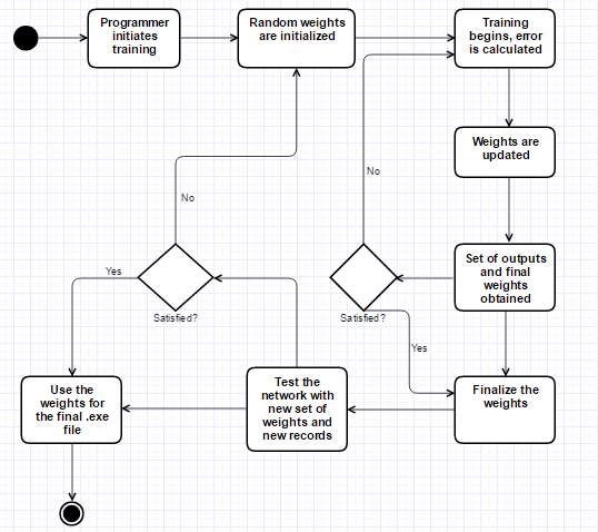
Figure 3.8 UML Diagram: State Chart diagram
State Chart diagrams are mainly used as a flow chart consists of activities performed by the system. But activity diagram are not exactly a flow chart as they have some additional capabilities. These additional capabilities include branching, parallel flow, swimlane etc.This State Chart diagram has some simple activities and the flow of data through conditional statements.
CHAPTER 4
IMPLEMENTATION
4.1 Modules
The implementation has been divided into 4 modules:
- Algorithm
- Feed Forward
- Training the Network
- Testing the Network
4.1.1 Algorithm
{
{
1. Import .csv file
2. Open the file using ‘genfromtxt’ method.
3. Data cleaning can be done if necessary.
}
4. Import numpy as np
5. Class NN :
{
6. Initialize inputs (self.x = x), outputs (self.y =y)
7. Initialize number of layers (layerCount), number of neurons in each layer
8. BuildNetwork Method ():
{
9. Initialize weights, biases randomly
10. Initilize input vector and output vector
11. While (each epoch ends or terminating condition doesn’t satisfy)
{
12. Initialize input with input parameters = x
FeedForward Method ():
For each neuron in hidden layer,
Sum = total summation of (x[i] * w[i][j])
Out[i][j] = sigmoid(sum)
}
Calculate the same for output layer
13. ErrorEstimation Method ():
E = ½ * (O[k] – t[k]) ^ 2
14. Minimize error by finding error derivative
Change in weight = tr * O[j] * Del[k], Del[k] = O[k](1 – O[k])(O[k] – t[k])
Change weights when required
15. Repeat the above process until terminating condition satisfies
}
}
16. Accept parameters from user and predict the new output
This algorithm was partially used to develop the code for building the Neural Network for predicting Diabetes.
This algorithm generally works for the basis of designing any Neural Network and coding in any programming language or scripting language.
4.1.2 Feed Forward
Any Neural Network when run, will display the output after mathematical calculations. We can compare the obtained output with the expected output and test the efficiency of the calculations. In the feed forward part, no training has been done and naturally, the outputs are not as we expect them to be.
Feed forward part of the code is plain matric multiplications of weights with the input data. In Python, according to the code written, weights are generated randomly in the beginning and are stored in a list of list. Later this list of list is converted into 2-D array and matrix multiplications will be done.
Below are the bar graphs of different sets of data, each containing 100 records where mathematical multiplications have been done without training the data.
Set 1 (100 records) –
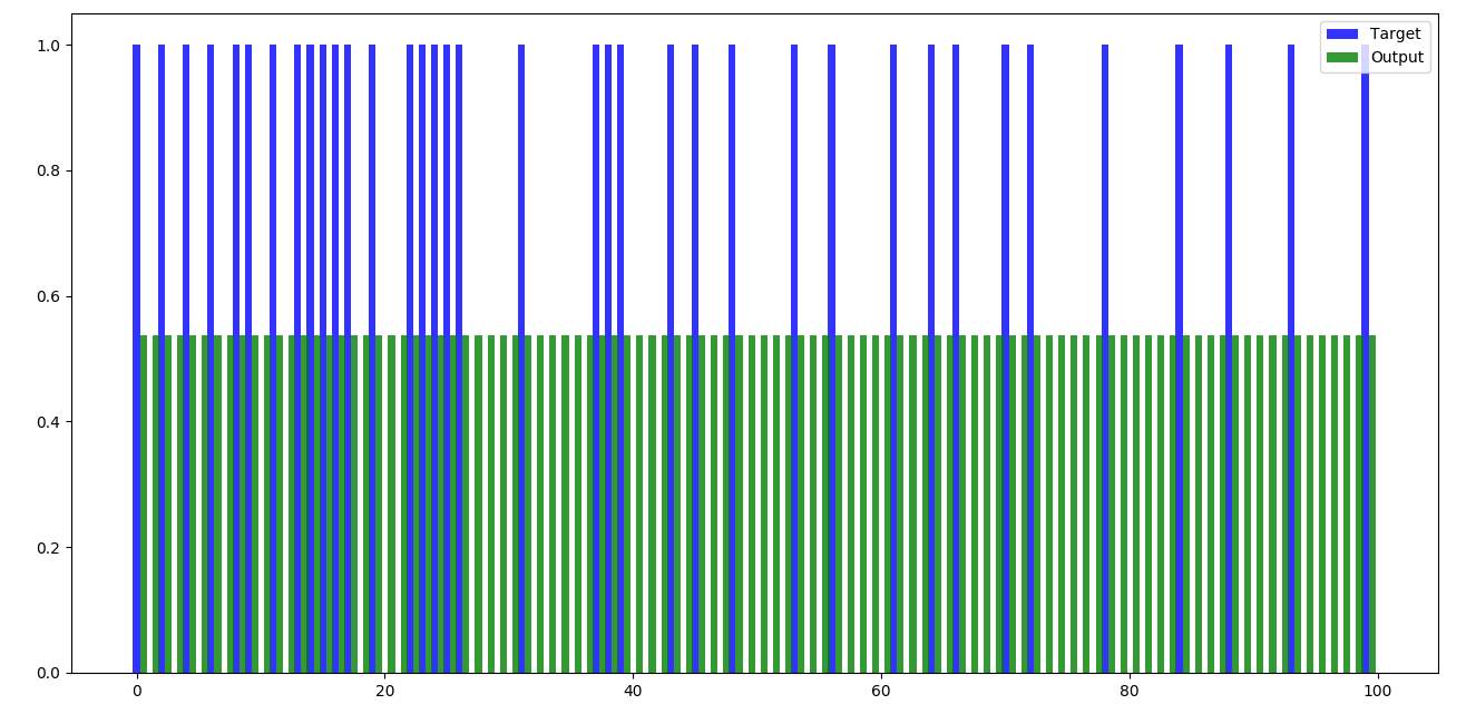
Figure 4.1 Feed forward – set 1
Set 2 (100 records) –
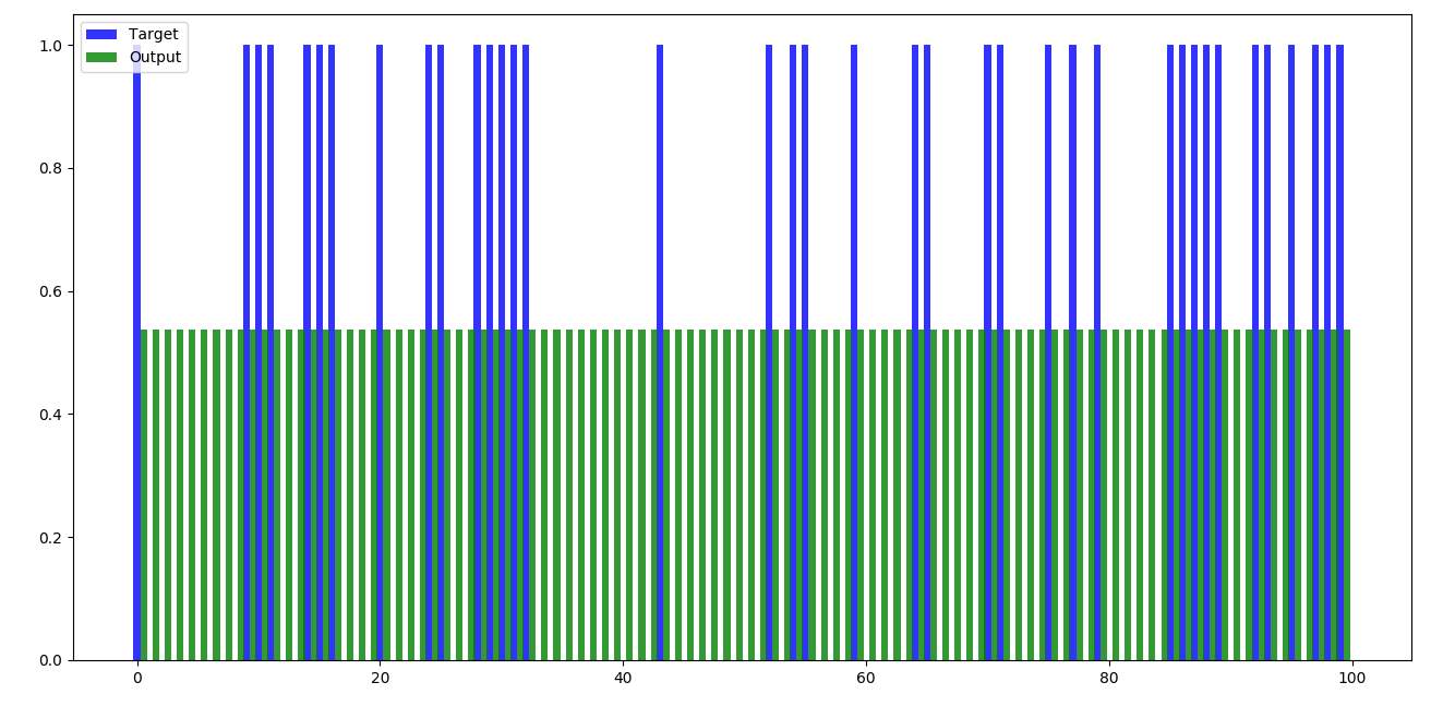
Figure 4.2 Feed forward – set 2
Set 3 (100 records) –
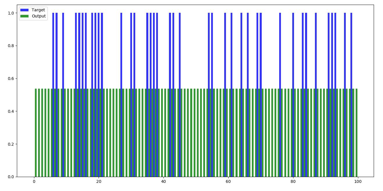
Figure 4.3 Feed forward – set 3
Set 4 (100 records) –
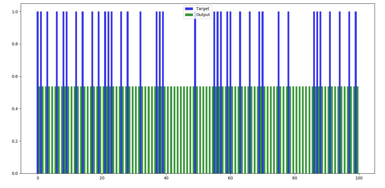
Figure 4.4 Feed forward – set 4
Set 5 (100 records) –
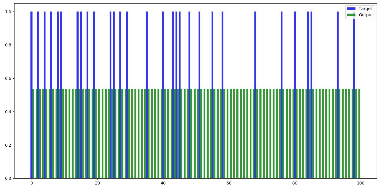
Figure 4.5 Feed forward – set 5
4.1.3 Training the Network
As we have seen in the previous section, the network has been giving horrible results because weights that were multiplied were only the randomly generated weights. They weren’t tested nor were trained. Hence, training should be done so that the error rate that has been obtained will be reduced and we get accurate results during training.
Training for 300 records has been done at a time and has been carried out for 2,50,000 iterations. We have trained the network 10 times only to obtain the average training error and accuracy to finalize the performance of the neural network.
Hence, 10 trials with Error vs Iteration graph, final error rate after 2,50,000 iteration and accuracy of the result will be shows for each trial.
Sample weight matrix: [array([[ 26.59723618, 14.18107419, 10.92878201, 26.85052849, 42.61233364, -19.27722132, -37.96911852, -64.48465948, 17.32754906],
[2.19300302, -0.99467817, -5.69296451, -5.27359341, -8.35276447, -5.16051119, -6.9926969 , 5.74247897, 7.27711032],
[47.67559925, 25.05766031, -23.17578356, -20.12256636, 3.89993303, -10.59420603, -33.50110588, -21.25992775, 4.39447616],
[-5.37264149, -16.28338031, -3.91462964, 6.02717533, 25.665084, -28.45946387, 3.2846802, -35.41830161, 31.48699416],
[20.20013048, 17.44072058, -7.98092068, 7.31561335, -26.11945465, -4.7767389, -29.92634953, 26.82968151, -4.29161374]]),
array([[-45.02923454, -95.82695757, 58.56097862, -41.686042 , 65.98056637, 4.89618671]])]
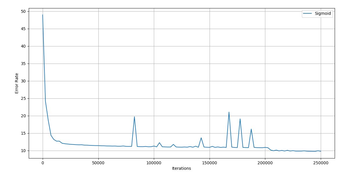
Figure 4.6 Sample Iteration vs Error graph
Trial 1 –

Figure 4.7 Trial 1 Iteration vs Error graph
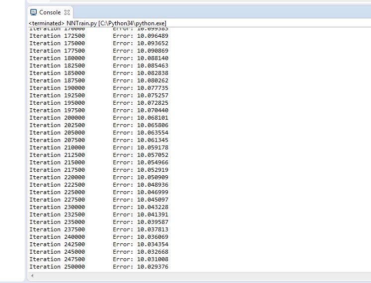
Figure 4.8 Trial 1 Error rate
Final error rate: 10.029
Accuracy of the trained network: 96.6%
Trial 2 –
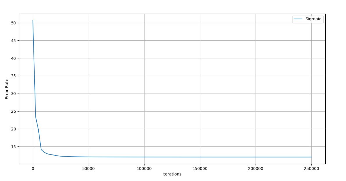
Figure 4.9 Trial 2 Iteration vs Error graph
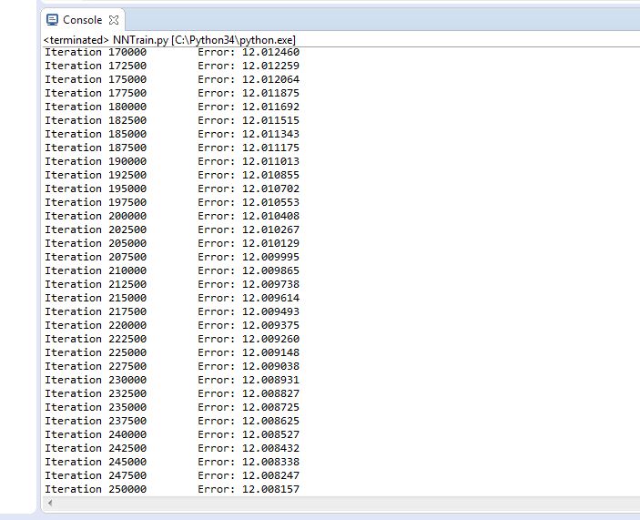
Figure 4.10 Trial 2 Error rate
Final error rate: 12.008
Accuracy of the network: 97%
Trial 3 –
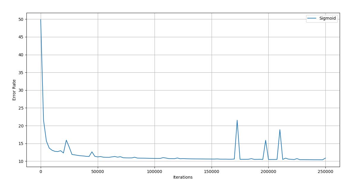
Figure 4.11 Trial 3 Iteration vs Error graph
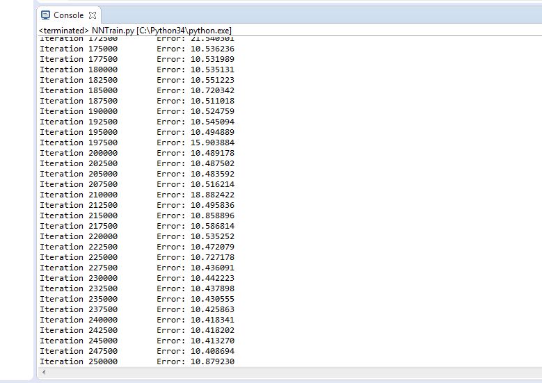
Figure 4.12 Trial 3 Error rate
Final error rate: 10.878
Accuracy of the network: 95%
Trial 4 –
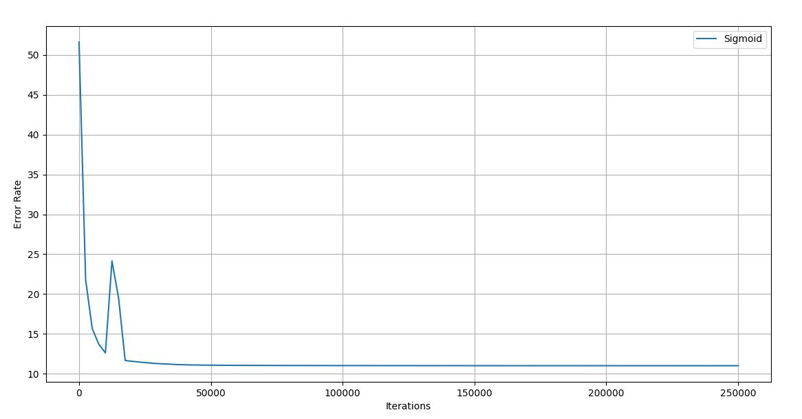
Figure 4.13 Trial 4 Iteration vs Error graph
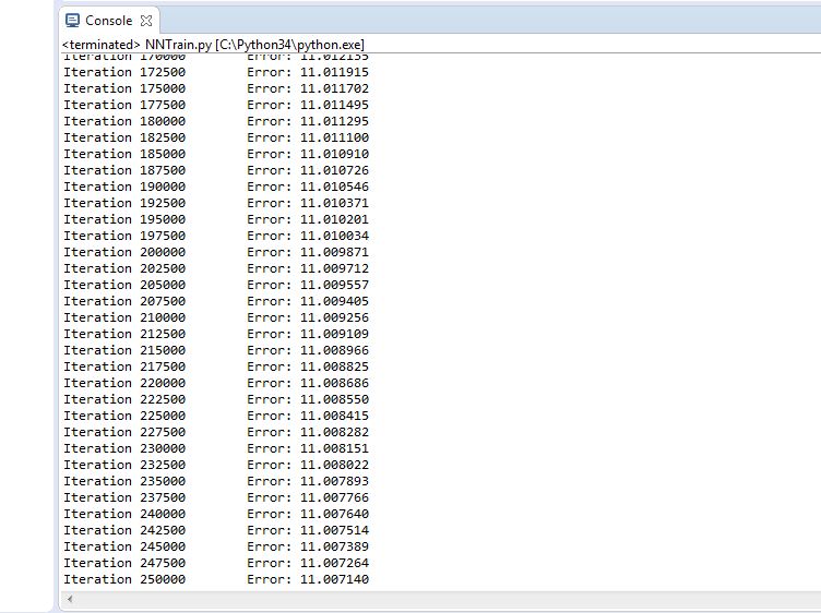
Figure 4.14 Trial 4 Error rate
Final error rate: 11.0077
Accuracy of the network: 95.3%
Trial 5 –
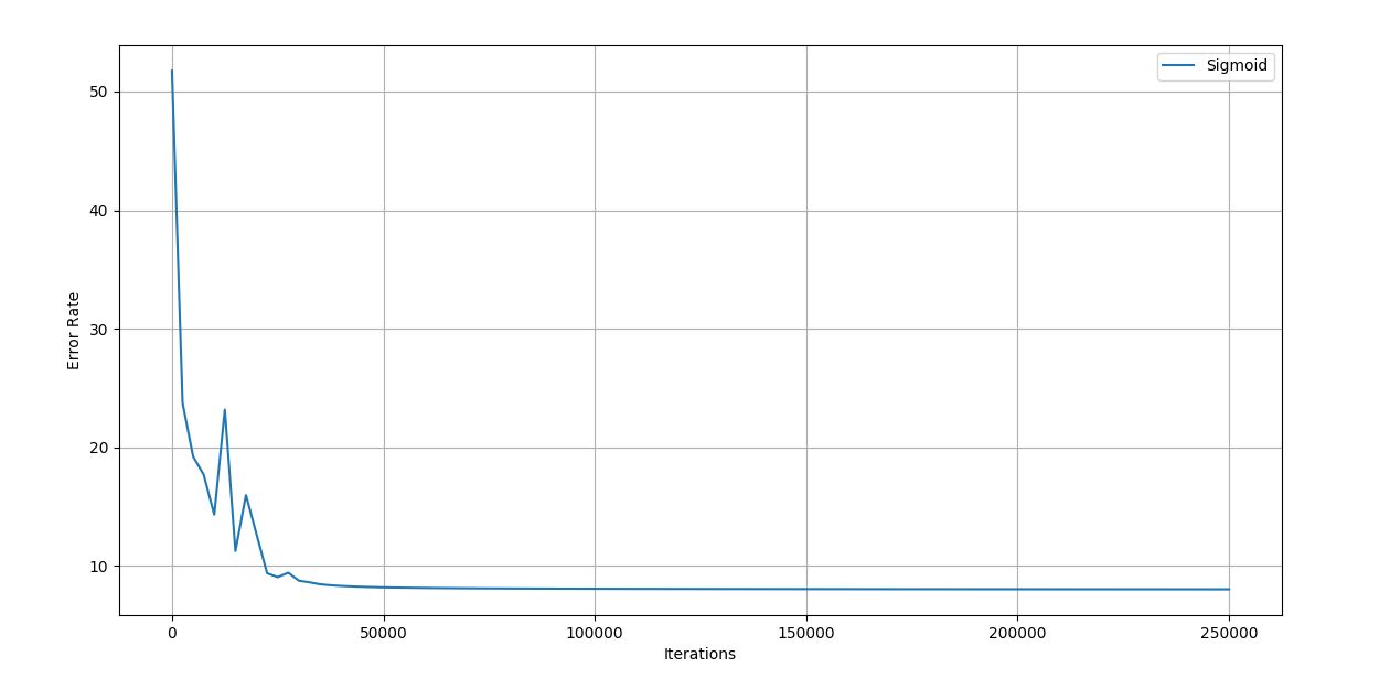
Figure 4.15 Trial 5 Iteration vs Error graph
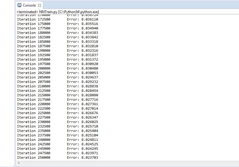
Figure 4.16 Trial 5 Error rate
Final error rate: 8.023
Accuracy of the network: 97%
Trial 6 –
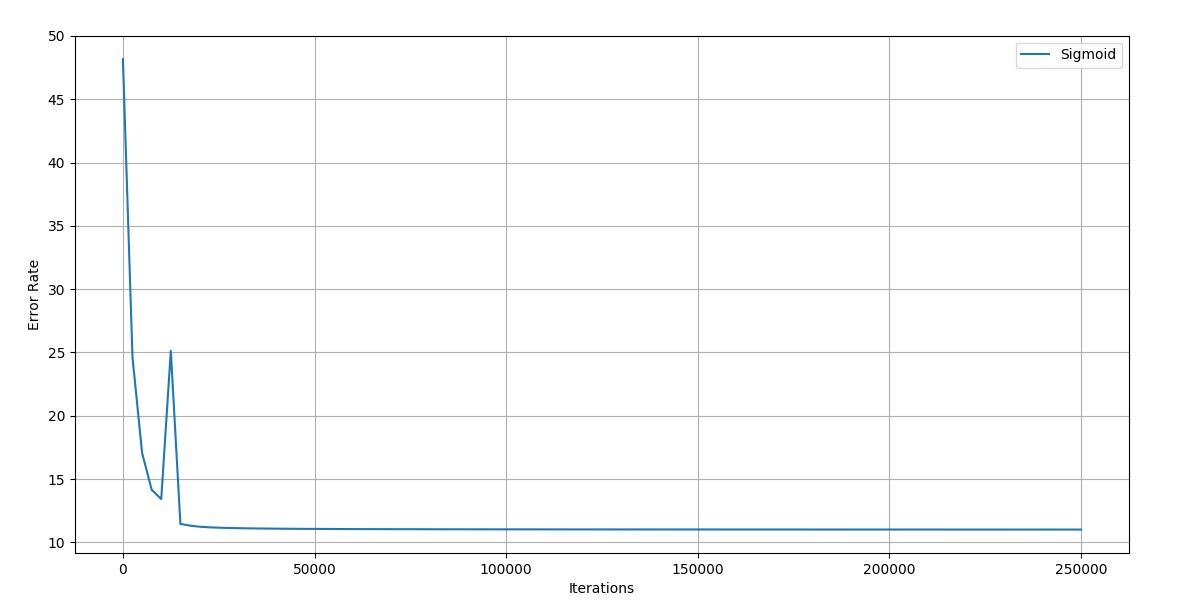
Figure 4.17 Trial 6 Iteration vs Error graph
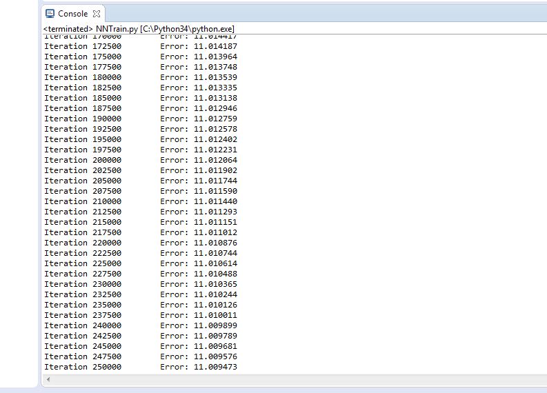
Figure 4.18 Trial 6 Error rate
Final error rate: 11.009
Accuracy of the network: 93.6%
Trial 7 –
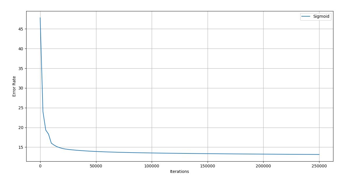
Figure 4.19 Trial 7 Iteration vs Error graph
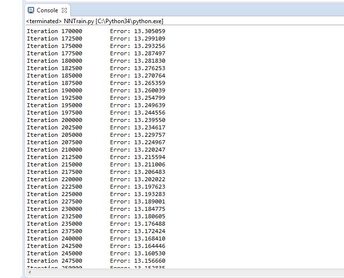
Figure 4.20 Trial 1 Error rate
Final error rate: 12.16
Accuracy of the network: 95.6%
Trial 8 –
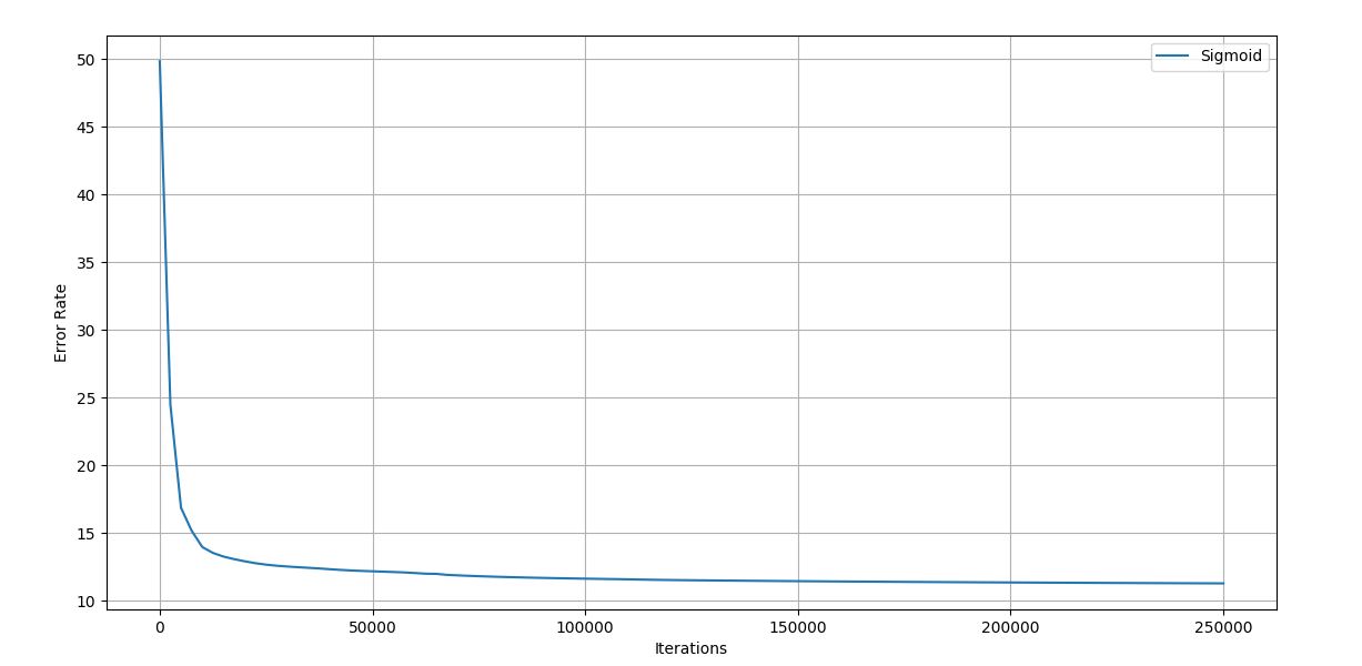
Figure 4.21 Trial 8 Iteration vs Error graph
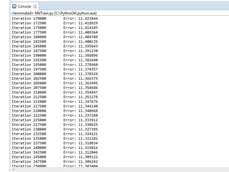
Figure 4.22 Trial 8 Error rate
Final error rate: 11.303
Accuracy of the network: 93.3%
Trial 9 –

Figure 4.23 Trial 9 Iteration vs Error graph
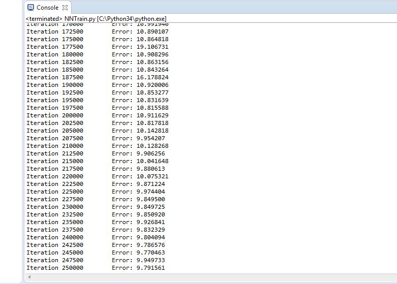
Figure 4.24 Trial 9 Error rate
Final error rate: 9.791
Accuracy of the network: 94.6%
Trial 10 –
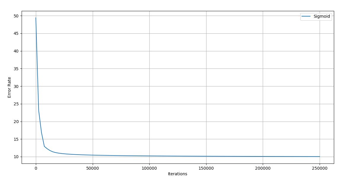
Figure 4.25 Trial 10 Iteration vs Error graph

Figure 4.26 Trial 10 Error rate
Final error rate: 10.029
Accuracy of the trained network: 96.6%
4.1.4 Testing the Network
After training has been done to the network, a final set of weights are obtained that should be used for testing the network because those are the corrected numbers according to the dataset and outputs given during supervised learning.
We have a dataset of 768 records, in which 500 have been iteratively and alternatively been used for training the network.
The remaining records are used for testing and out of which, 10 records have been chosen.
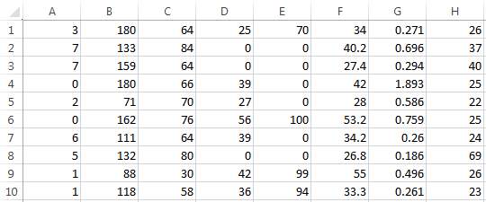
Dataset for testing
The corresponding outputs for these records is as follows:
| 0 |
| 0 |
| 0 |
| 1 |
| 0 |
| 1 |
| 0 |
| 0 |
| 1 |
| 0 |
Where, 0 stands for not diabetic and 1 stands for diabetic.
After passing these records into the testing part of the code, the results obtained are:
| [ 9.99987966e-05] |
| [ 3.94139766e-19] |
| [ 9.99999731e-01] |
| [ 5.23674871e-20] |
| [ 5.00000000e-01] |
| [ 9.98454055e-01] |
| [ 1.00000000e+00] |
| [ 8.66186436e-12] |
| [ 0.99028980e-01] |
| [ 9.47488430e-36]] |
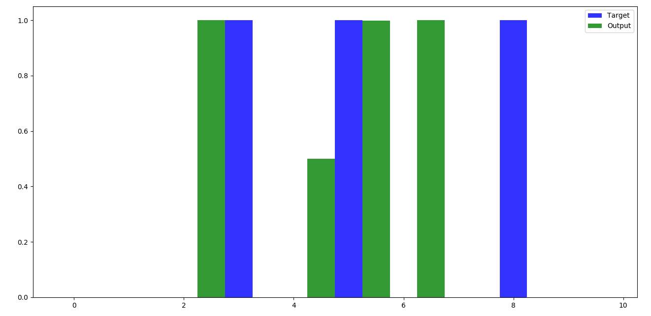
Figure 4.27 Graph obtained after testing
This means that 7 out of 10 records have been classified correctly during testing and this makes the model 70% accurate.
4.2 Code Snippets
This software project has been coded in Python programming language.
4.2.1 Feed Forward Network
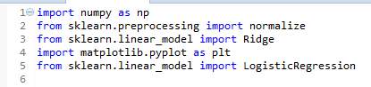
Figure 4.28 Libraries used
The above image describes the Python packages used and below image shows the part of code that perform the feed forward operation.
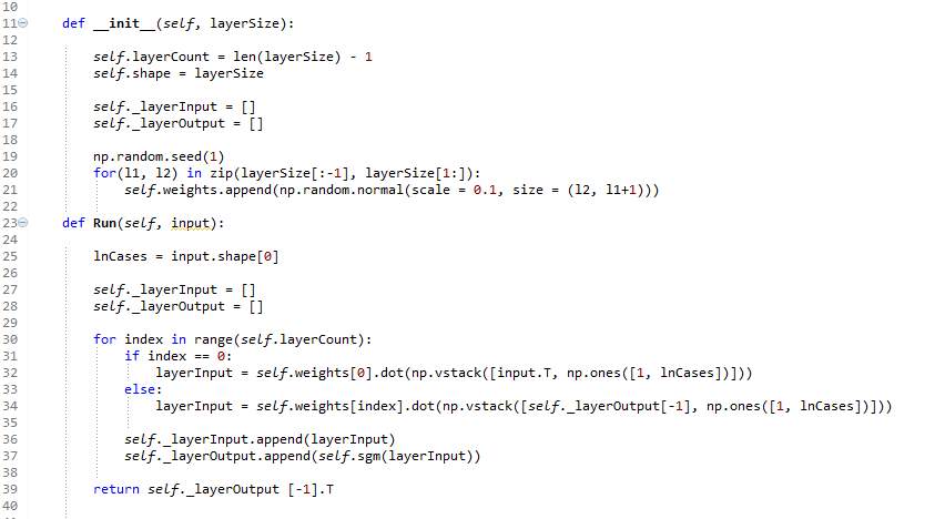
Figure 4.29 Feed forward code
4.2.2 Training Method
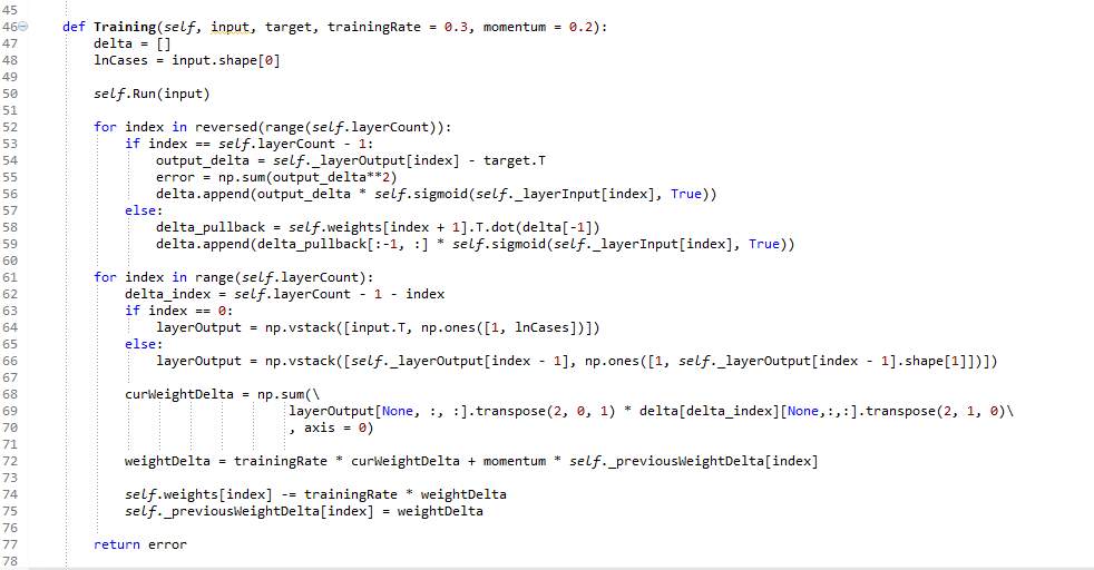
Figure 4.30 Training Code
4.2.3 Testing Method
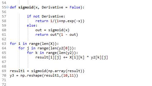
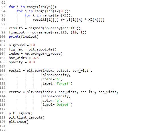
Figure 4.31 Testing code
4.3 Introduction to Technologies
The project that has been built has been using many technologies and softwares to work. The Neural Network has been realized in programming language Python and implemented in a software called PyDev.
The list of softwares and modules used are:
- Java 8
- Eclipse Neon
- Python Interpreter v3.4
- Numpy 1.12
- Scipy 0.19
- Scikit
- Matplotlib
- PyDev console for Eclipse
- Neural Designer
- Python to .exe converter
4.3.1 Java 8

Figure 4.32 Java logo [51]
Java is an object-oriented language which is similar to C++, but is simple enough to abate any language functions that can cause common errors in programming. The code files have an extension of .java. These are compiled into a format known as bytecode. This format can be executed by a Java interpreter (JI). The compiled code can work on most of the present day platforms and computers because Java runtime environments and interpreters, known as Java Virtual Machines (JVMs), exist in most operating systems, including the Macintosh OS, UNIX, and Windows. Bytecode which has an extension of .class, can be transformed directly, into instructions of machine language by a compiler called Just-In-Time (JIT). It is considered to be more reliable than many programming languages because of its security reasons, reliability and robustness.
Since the inception, a number of versions of Java have been released. Java 8 is one of the versions that we have used [20].
- JDK Alpha and Beta
- JDK 1.0
- JDK 1.1
- J2SE 1.2
- J2SE 1.3
- J2SE 1.4
- J2SE 5.0
- Java SE 6
- Java SE 7
- Java SE 8
- Java SE 9
- Java SE 10
Java 8 is installed on the system as Eclipse IDE works only with proper working of Java 8 version.
4.3.2 Eclipse Neon
Eclipse is an integrated development environment (IDE) used in programming which is widely used a Java IDE. It competes with another IDE known as Android studio. It contains an extensible plug-in system and an established base workspace for customizing efficiently, the environment. Eclipse is primarily written in Java and some other programming languages and its significant use is for creating developing and modifying applications in Java. However, it can also be used to create and develop applications in many other programming languages through plug-ins. These include Ada, ABAP, C, C++, Prolog, COBOL, D, NATURAL, Clojure, Perl, PHP, Groovy, Python, R, Ruby (which includes the framework of Ruby on Rails), Scheme, and Erlang [21].

Figure 4.33 Eclipse logo [52]
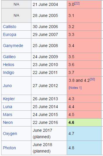
Figure 4.34 Eclipse versions [53]
We are using Eclipse Neon 4.6 for this implementation.
4.3.3 Python Interpreter v3.4

Figure 4.35 Python logo [54]
Python, released in 1991, is known as a general-purpose programming language which is high level in nature. It is also an open source programming language, which is very much widely used across many people around the world. It is an interpreted language which has not only has a stunningly innovative design philosophy that specializes on the readability of the code, but also contains a syntax that allows various programmers to effectively express their problems in much lesser lines of code in languages like Java or C++. The language provides details necessary to provide writing vivid programs in large and even small scale. Python features an innovative type system which is dynamic in nature and automatic facility of memory management and supports multiple programming paradigms, including functional and object oriented programming and various methods in procedural analysis. It has a large and comprehensive standard library. Python interpreters of different versions are available for many operating systems like Windows, Mac OS, etc., enabling the code to work on a wide range of systems [22].
One can check the Python version at the command line by running python –version.
In computer science, an interpreter is a computer program that directly executes the code, i.e. performs, instructions written in a programming or scripting language, without previously compiling them into a machine language program. An interpreter generally uses one of the following strategies for program execution:
- parse the source code and perform its behavior directly.
- translate source code into some efficient intermediate representation and immediately execute it.
- explicitly execute stored precompiled code made by a compiler which is part of the interpreter system [23].
Release dates for the major and minor versions:
- Python 1.0 – January 1994
- Python 1.5 – December 31, 1997
- Python 1.6 – September 5, 2000
- Python 2.0 – October 16, 2000
- Python 2.1 – April 17, 2001
- Python 2.2 – December 21, 2001
- Python 2.3 – July 29, 2003
- Python 2.4 – November 30, 2004
- Python 2.5 – September 19, 2006
- Python 2.6 – October 1, 2008
- Python 2.7 – July 3, 2010
- Python 3.0 – December 3, 2008
- Python 3.1 – June 27, 2009
- Python 3.2 – February 20, 2011
- Python 3.3 – September 29, 2012
- Python 3.4 – March 16, 2014
- Python 3.5 – September 13, 2015
- Python 3.6 – December 23, 2016
Python is a programming and scripting language which is very flexible and robust in nature. It has a large set of libraries and can be installed into the system using either Anaconda or PIP. The libraries that were used for out project are Numpy, Scipy, Scikit and Matplotlib.
- 4.3.3.1Numpy v1.12

Figure 4.36 Numpy logo [55]
NumPy is an array-processing package and library which is general-purpose innature. It is designed to effectively modify and calculate large arrays of multi-dimensions and arbitrary records. These are done quickly without consuming much time for small multi-dimensional arrays. NumPy software is developed on the code base of Numeric standard and extends features introduced by NumPy-array. It also has the ability to develop arrays of the arbitrary type. .NumPy is efficiently reliable for interfacing with applications of general-purpose data-base. The set of mathematical functions available in python are of many types: Trigonometric functions, floating points, Hyperbolic functions, Sum, product, complex functions, logarithmic and exponential functions, arithmetic functions, Rounding offs, special functions, differences, etc [24].
The functions used by us in this implementation are:
- Numpy.exp
- Numpy.array
- Numpy.reshape
- Numpy.arange
- Numpy.dot
- Numpy.genfromtxt
- Numpy.append
- Numpy.random
It can be install on the system by opening the Command Prompt and run it in Administrator mode. Next, type Pip install Numpy and see all the files automatically being installed in the system.
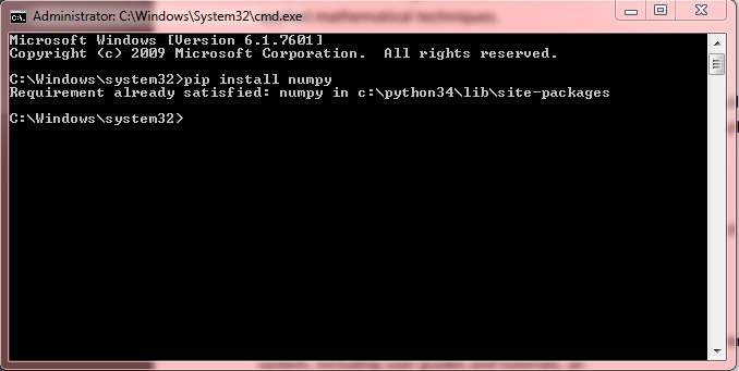
Figure 4.37 Numpy installation
- 4.3.3.2 Scipy v0.9

Figure 4.38 Scipy logo [56]
SciPy stands for Scientific Python. As the name suggests, it is an open source Python library. It is primarily used for scientific and technical computing. It. SciPy consists modules for many significant processes like signal and image processing, integration, linear algebra, optimization, regularization and many other tasks. It is also used for tasks which are very common in science and engineering. SciPy is formed on the basis of the array objects of NumPy and is an essential component of the NumPy stack which is also sometimes referred to as the SciPy stack. This also includes tools like SymPy and Matplotlib and many more. There is large library set in scientific computing that is added to the NumPy stack. This has users similar to a number of widely used applications such as GNU Octave, Matlab, and Scilab. [25].
To install SciPy on Windows, we need to follow the steps same as that of NumPy.
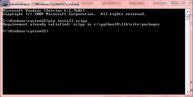
Figure 4.39 Scipy installation
- 4.3.3.3 Scikit

Figure 4.40 Scikit learn logo [57]
Scikit-learn (formerly scikits.learn) is a special and free software machine learning library for the Python programming language. It features and supports various classification, regression and clustering algorithms including support vector machines, random forests, gradient boosting, k-means and DBSCAN, and is designed to interoperate with the Python numerical and scientific libraries NumPy and SciPy [26].
This is used in the project to use function “Normalize” to normalize the input data from file.
- 4.3.3.4 Matplotlib
Figure 4.41 Matplotlib logo [58]
Matplotlib is a Python 2D and 3D plotting library which produces publication and quality figures in a variety of hardcopy formats and interactive environments across various platforms. Matplotlib can be used in Python scripts, the Python and IPython shell, the Jupyter notebook, web application servers, and four graphical user interface, Matlab applications, etc. toolkits.matplotlib.pyplot is a collection of command style functions that make matplotlib work like MATLAB. Each pyplot function makes some changes to a figure: e.g., creates a graphical figure, creates a graph plotting area in a figure, plots some lines in a plotting area, decorates the plot with labels, legends, etc. In matplotlib.pyplot various states are preserved across different function calls, so that it can keep track of things like the current figure of usage and plotting area, and the plotting functions are directed to the current axes [27].
4.3.4 Pydev for Eclipse
PyDev is a third-party plug-in for Eclipse. It is an Integrated Development Environment (IDE) used for programming in Python supporting graphical debugging, code refactoring, code analysis among other features [28].

Figure 4.42 PyDev logo [59]
Figure 4.43 PyDev console
4.3.5 Neural Designer
Neural Designer is a software tool for advanced data analytics based on neural networks, a main area and field of artificial intelligence research. It is developed from the very famous open source library made for neural networks, OpenNN, and contains a graphical user interface, GUI which simplifies data entry and interpretation of results.

Figure 4.44 Neural Designer logo [60]
Neural Designer performs descriptive, diagnostic, predictive and prescriptive data analytics. It implements deep architectures with multiple non-linear layers and contains utilities to solve function regression and classification, pattern recognition, time series, data description, structure generation and auto-encoding problems. The input to Neural Designer is a data set, and the output from it is a predictive model. That result takes the form of an explicit mathematical expression which can be exported to any computer language or system, especially to Python language and Python interpreters. We used this software to design the structure of the Neural Network with vivid difference among the layers [29].
Note: Few other sources were referred for learning the working of Neural Networks and the nature of Diabetes diseases. Sources like:
YouTube tutorials [30],[31],[32],
UCI repository [33],
Github links [34],[35][36],
Creately drawing platform [37],
Online courses from reputed institutions [38],
Eclipse and other software installation references [39] and
Executable file converters [40]
CHAPTER 5
TESTING
5.1 Introduction
Every software module or script or implementation must be tested with various cases and examples before deploying it to the customer who requires the software for usage. If there are any bugs or if the result is not satisfactory, the programmer must ensure to reduce anomalies to minimum before deploying.
5.2 Test Cases and Screenshots
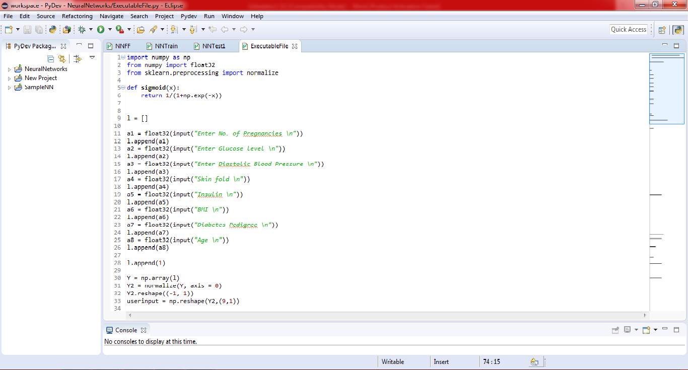
Figure 5.1 Final test code – 1
The above part of code scans inputs from the user and stores them in a list. Later, this list is converted into 1-D array of elements ready for matrix multiplication.
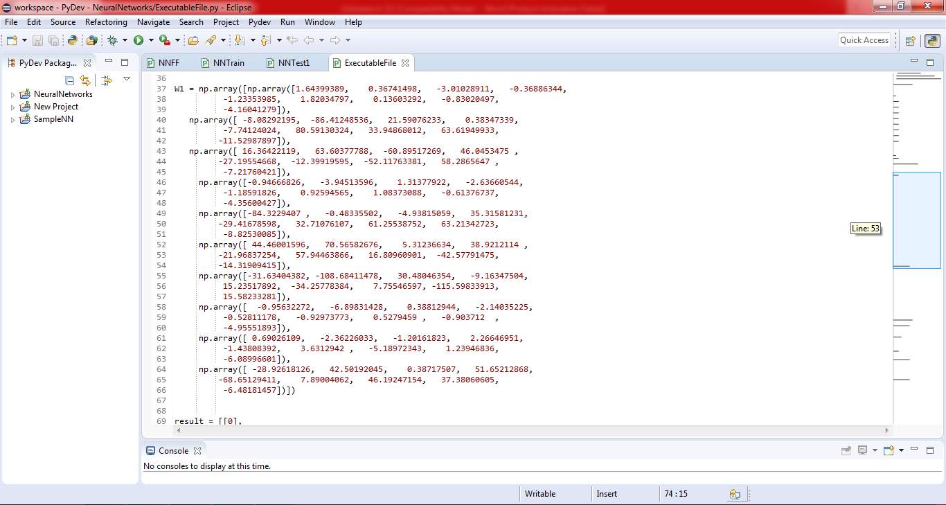
Figure 5.2 Final test code – 2
This part of the code has a list of lists containing the final set of weights that has been decided after training the network.
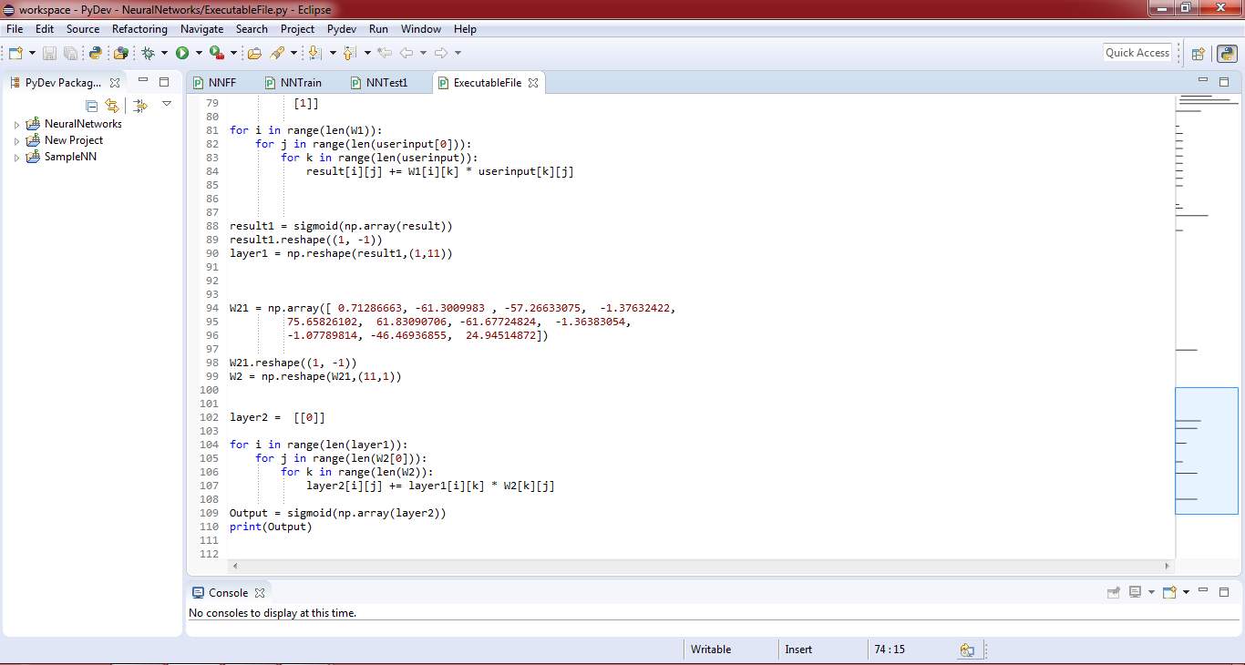
Figure 5.3 Final test code – 3
This part of the code shows the multiplication steps between input matrix and weight matrices.
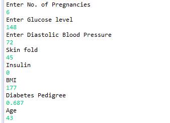
Figure 5.4 Inputs given to the network
[9.10833313e-05] is the output generated by the network, which can be considered 0. It means, the person who entered values with those attributes is not in a danger of being diabetic.
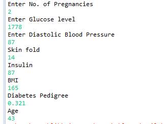
Figure 5.5 Input given to the network
[7.48323813e-06] is the output generated by the network, which can be considered 0. It means, the person who entered values with those attributes is not in a danger of being diabetic.
CHAPTER 6
CONCLUSION
Diabetes is one of the most common health issue seen in the present times. Taking proper care of oneself by adapting to a healthy lifestyle is the key to keep not only diabetes but all other health hazards at bay. In our project report titled “Diabetes prediction using neural networks”, we have strived to present an efficient and intelligent prediction method using neural networks following the motto “Prevention is better than cure.”
Neural network is a powerful tool for performing diagnosis as it can process large amounts of input data quickly and thoroughly. This results in reduction of processing time and mistaken overlooking of relevant information.
We have developed our trained neural net structure with 8 input layers, 10 hidden layers, 1 output layer and backed on back propagation. Back propagation algorithm is the most preferred algorithm amongst all others due to its bankable and accurate processing trait.
Greater efforts can be put towards the improvement of our system so as to enhance its precision, efficiency and swift result obtaining capabilities.
Using neural network structure, checking for diabetes can be done quickly and painlessly without shelling out any additional costs for other tests.
This prediction system would be a boon in the field of medical wellness as many medical professionals could plan a better customized medication chart for each patient in early stages itself and obtain greater improvement in the health and fitness aspect.
CHAPTER 7
FUTURE ENHANCEMENTS
Application of the neural networks for diagnosis of various diseases like diabetes is the next big thing in the medical field. With proper exposure to the benefits of using machine learning techniques in the diagnosis of patients, we expect the leading hospitals in our country to implement the technology.
The major aim of our project is to aid a person in knowing the likelihood of him being diagnosed with diabetes so that he could take the necessary care to avoid it.
Our code could be converted to an executable file which could be shared through the internet so that anyone can install and run it.
Our code could be embedded into an application which will be connected to the electronic fitness band which will track the necessary vitals of the person. This application will take inputs from the person directly without the manual entry and will give the predicted output.
The performance of the code could be increased with the application of proper optimization techniques.
REFERENCES
[1] Ms. Divya, Raman Chhabra, Sumit Kaur, Swagata Ghosh, “Diabetes Detection Using Artificial Neural Networks & Back-Propagation Algorithm”, International Journal of Scientific and Technology Research, Volume 2, Issue 1, January 2013. http://www.ijstr.org/
[2] Scott M. Pappada, Brent D. Cameron, Paul M. Rosman, “Development of a Neural Network for Prediction of Glucose Concentration in Type 1 Diabetes Patients”, Journal of Diabetes Science and Technology Volume 2, Issue 5, September 2008.
[3] Hasan Temurtas, Nejat Yumusak, Feyzullah Temurtas, “A comparative study on diabetes disease diagnosis using neural networks”, Expert Systems with Applications 36 (2009) 8610–8615
[4] Jaafar, S. F. & Ali, D. M. (2005). “Diabetes Mellitus forecast using Artificial Neural Network” Paper presented at the Asian Conference on Sensors and the International Conference on New Techniques in Pharmaceutical and Biomedical Research.
[5] Prof. Sumathy, Prof. Mythili, Dr. Praveen Kumar, Jishnujit T M and Ranjith K Kumar, “Diagnosis of Diabetes Mellitus based on Risk Factors” International Journal of Computer Applications 10(4):1–4, November 2010.
[6] Jin Park and D. Edington, “A sequential Neural Network Model for Diabetes Prediction”, University of Michigan.
[7] B. Sumathi, Dr. A. Santhakumaran, “Pre-Diagnosis of Hypertension Using Artificial Neural Network”, Global Journal of Computer Science and Technology, Volume 11 Issue 2 Version 1.0 February 2011.
[8]Meenakshi Verma, “Medical Diagnosis using Back Propagation Algorithm in ANN”, International Journal of Science, Engineering and Technology Research (IJSETR), Volume 3, Issue 1, January 2014
[9] Machine Learning, https://en.wikipedia.org/wiki/Machine_learning
[10] Supervised Learning, http://machinelearningmastery.com/supervised-and-unsupervised-machine-learning-algorithms/
[11] Artificial Neural Networks, https://en.wikipedia.org/wiki/Artificial_neural_network
[12] Supervised Learning, http://machinelearningmastery.com/supervised-and-unsupervised-machine-learning-algorithms/
[13] Attributes of Neural Networks, https://en.wikibooks.org/wiki/Artificial_Neural_Networks/Neural_Network_Basics
[14] Activation Functions, https://en.wikipedia.org/wiki/Activation_function
[15] Optimization Algorithms, https://www.neuraldesigner.com/blog/5_algorithms_to_train_a_neural_network
[16] Over-fitting and Under-fitting, http://machinelearningmastery.com/overfitting-and-underfitting-with-machine-learning-algorithms/
[17] Problem statement for Diabetes Prediction, https://deepblue.lib.umich.edu/bitstream/handle/2027.42/75845/hagan_3.pdf%3Fsequence%3D1
[18] SRS Document, https://en.wikipedia.org/wiki/Software_requirements_specification
[19] UML Diagrams basics, https://www.tutorialspoint.com/uml/uml_overview.htm
[20] Java, http://www.webopedia.com/TERM/J/Java.html
[21] Eclipse software, https://en.wikipedia.org/wiki/Eclipse_(software)
[22] Python programming, https://en.wikipedia.org/wiki/Python_(programming_language), https://www.python.org/downloads/, https://docs.python.org/3/
[23] Interpreter meaning, https://en.wikipedia.org/wiki/Interpreter_(computing)
[24] NumPy Documentation, https://engineering.ucsb.edu/~shell/che210d/numpy.pdf, http://cs231n.github.io/python-numpy-tutorial/, https://docs.scipy.org/doc/numpy/reference/, https://pypi.python.org/pypi/numpy/1.6.1
[25] SciPy Documentation, https://en.wikipedia.org/wiki/SciPy
[26] Scikit-learn Documentation, https://www.datacamp.com/community/tutorials/machine-learning-python#gs.=c7zo=Q, http://scikit-learn.org/stable/
[27] Matplotlib, PyPlot documentation, http://matplotlib.org/users/pyplot_tutorial.html
[28] PyDev Documentation, https://wiki.python.org/moin/PyDev, http://www.pydev.org/
[29] Neural Designer, https://en.wikipedia.org/wiki/Neural_Designer
[30] Welch Labs (Neural Networks), https://www.youtube.com/results?search_query=welch+labs+neural+networks
[31] Ryan Harris (Neural Networks), https://www.youtube.com/watch?v=XqRUHEeiyCs&list=PLRyu4ecIE9tibdzuhJr94uQeKnOFkkbq6
[32] Siraj Raval (Neural Networks), https://www.youtube.com/watch?v=h3l4qz76JhQ&list=PL2dafEMk2A5BoX3KyKu6ti5_Pytp91sk
[33] UCI Repository, Pima Indians Diabetes, https://archive.ics.uci.edu/ml/datasets/Pima+Indians+Diabetes
[34] Github, https://github.com/TheFellow/Neural-Network-Tutorial-Python
[35] Github, https://github.com/stephencwelch/Neural-Networks-Demystified
[36] Github, https://github.com/kjw0612/awesome-rnn
[37] Creately platform, https://creately.com/app/?tempID=ildfq2zd5&login_type=demo#
[38] Online courses, https://www.coursera.org/
[39] Eclipse and Pydev installation, https://www.ics.uci.edu/~pattis/common/handouts/pythoneclipsejava/eclipsepython.html
[40] Executable file converters, https://www.google.co.in/webhp?ei=oYQBWYKZE8uNvQTbnJnwDw&yv=2&rct=j#q=convert+python+3.4+to+exe
[41] Machine Learning, http://img.deusm.com/informationweek/2016/08/1326571/machine-learning-NicoElNino-iStock_96316291_MEDIUM.jpg
[42] Machine Learning, https://static.wiliam.com.au/assets/2016/09/blog-featured-10589-MachineLearning.jpg
[43] General Structure of Neural Network, https://upload.wikimedia.org/wikipedia/commons/thumb/4/46/Colored_neural_network.svg/300px-Colored_neural_network.svg.png
[44] Example of Neural Network Applications, Thompson Scattering Experiment, http://iopscience.iop.org/article/10.1088/0741-3335/55/9/095015
[45] Perceptron Structure, https://www.tutorialspoint.com/artificial_neural_network/images/perceptron.jpg
[46] Location of Perceptron in a typical Neural Network, Another representation of Perceptron, Weights on synapses, Error reduction by finding global minimum, One dimensional optimization, Five types of optimization techniques, Flow-chart of Gradient Descent algorithm, https://www.neuraldesigner.com/blog/perceptron-the-main-component-of-neural-networks
[47] Back Propagation algorithm, https://tex.stackexchange.com/questions/162326/drawing-back-propagation-neural-network
[48] Problems faced during training a Neural network, https://datascience.stackexchange.com/questions/361/when-is-a-model-underfitted
[49] Types of fitting problems in Neural Networks, http://vitalflux.com/machine-learning-diagnose-underfittingoverfitting-learning-algorithm/
[50] Types of SRS, https://www.tutorialspoint.com/software_testing_dictionary/software_requirement_specification.htm
[51] Java logo, http://www.smissltd.com/blog/date-and-time-api-java-8
[52] Eclipse logo, https://eclipse.org/artwork/
[53] Eclipse versions, https://wikipedia.org/Eclipse-versions
[54] Python logo, http://www.pngall.com/python-logo-png
[55] Numpy logo, https://bids.berkeley.edu/research/numpy
[56] Scipy logo, https://github.com/donnemartin/data-science-ipython-notebooks
[57] Scikit learn logo, https://github.com/scikit-learn/scikit-learn
[58] Matplotlib logo, http://matplotlib.org/1.2.1/examples/pylab_examples/histogram_demo.html
[59] PyDev logo, https://en.wikipedia.org/wiki/File:Pydev_logo.png
[60] Neural Designer logo, https://commons.wikimedia.org/wiki/File:Neural_Designer_logo.png
Cite This Work
To export a reference to this article please select a referencing stye below:
Related Services
View all


Related Content
All TagsContent relating to: "Biology"
Biology is the scientific study of the natural processes of living organisms or life in all its forms. including origin, growth, reproduction, structure, and behaviour and encompasses numerous fields such as botany, zoology, mycology, and microbiology.
Related Articles

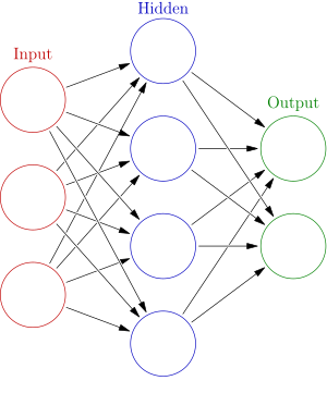
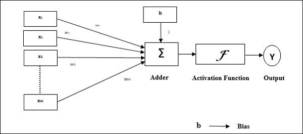
DMCA / Removal Request
If you are the original writer of this dissertation and no longer wish to have your work published on the UKDiss.com website then please: