Hidden Surface Removal Using Binary Space Partitioning
Info: 8927 words (36 pages) Dissertation
Published: 25th Aug 2021
Tagged: Computer Science
ABSTRACT
“BSP”- Binary Space Partitioning is a project which is going to deal with the complexity of space division,
Binary Space Partitioning is a method of recursively subdividing a space into convex sets using hyper planes. BSP uses tree data structure to store information about set of objects in each convex set. The whole BSP tree is constructed as a pre-processing step and at the time of program runs, the tree is processed at each run to calculate that which division space we are interacting with at runtime.
The main purpose for doing this project is to understand the concept of BSP and using it we implement one of its application i.e. hidden surface removal which can be described as- while playing Games we are unable to see the full map / scene in one time only the camera perspective is visible. In this case if the whole map is rendered then it is a waste, as well as our GPU is also heavily consumed. So, we need to render only that part of map which is currently in the camera perspective. This would lead to fewer loads on GPU and efficient performance, no wastage of memory.
The process uses recursive approach. A single super space is divided into 2 subspaces by a hyper plane, and then the 2 subspaces are treated as super spaces and further divided into 2 subspaces. This process is followed until each object is in separate subspace.
Keywords: Binary Space Partitioning, Complexity, Hidden surface removal, Visible Surface Detection, algorithm
TABLE OF CONTENTS
| S. no. | Contents | Page no. |
| 1. | Introduction | 7 |
| 1.1 | BSP and BSP Trees | 8 |
| 1.2 | Problem Statement | 9 |
| 2. | Literature Review | 10 |
| 2.1 | On Visible Surface Generation By A Priori Tree Structures | 10 |
| 2.2 | Predetermining Visibility Priority In 3-D Scenes | 12 |
| 2.3 | Optimization Of The Binary Space Partition Algorithm (Bsp) For The Visualization Of Dynamic Scenes | 13 |
| 3. | Key Concepts | 14 |
| 3.1 | Node | 14 |
| 3.2 | Tree | 15 |
| 4 | Model | 16 |
| 5 | Algorithm | 20 |
| 5.1 | Split function | 20 |
| 5.2 | Recursive Split function | 23 |
| 6 | Result and Discussion | 25 |
| 6.1 | Problems | 25 |
| 6.2 | Variations and Methods | 26 |
| 6.3 | Results | 34 |
| 7 | Conclusion | 35 |
| 8 | References | 36 |
TABLE OF FIGURES
| S.no. | Title | Page |
| 1 | Introduction | |
| 1.1 | A BSP-tree example | 8 |
| 2 | Literature Review | |
| 2.1 | Tree making process | 11 |
| 2.2 | B-rep and tree representation of BSP | 12 |
| 3 | Key Concepts | |
| 3.1 | Code snippet for BSPnode | 14 |
| 3.2 | A complex BSP | 15 |
| 4. | Model | |
| 4.1 | Zero iteration region | 16 |
| 4.2 | One iteration regions | 17 |
| 4.3 | Two iteration regions | 18 |
| 4.4 | Three iteration regions | 19 |
| 5 | Algorithm | |
| 5.1 | Recursive split function | 24 |
| 6 | Result and Discussion | |
| 6.1 | Back Face detection | 27 |
| 6.2 | Z-Buffer or Depth Buffer algorithm | 28 |
| 6.3 | Scanline | 29 |
| 6.4 | Painter’s algorithm 1 – idea | 30 |
| 6.5 | Painter’s algorithm 2 – execution | 30 |
| 6.6 | Octrees | 31 |
| 6.7 | A-buffer algorithm 1- idea | 32 |
| 6.8 | A-buffer algorithm 2- execution | 32 |
| 6.9 | Ray-casting orthogonal and perspective views | 33 |
| 6.10 | Ray-casting from 3D to 2D | 33 |
| 7 | Conclusion | |
| 7.1 | Output code of BSP | 35 |
INTRODUCTION
This report describes the results of implementation of Binary Space Partitioning for rendering of objects as images. For the graphical scenes the proposed algorithm also performs visible surface detection on a simple level which can be further used for hidden surface removal.
BSP and BSP Trees
BSP
In most applications generating images of 3D objects are crucial operations. Performing these operations in which more than 2 objects are present in a scene requires a check that the two objects might intersect each other or the occlude each other. However rather than being monolithic, objects appears to be comprised of many pieces, such as many polygons forming the image. So that if any piece of the image is intersecting or being overlapped by piece of another image then that piece of image should not be rendered. Computing spatial relations between n polygons following the brute force approach require comparing every pair, so would require O(n2). This would be so complex for large no of polygons.
The above number could be reduced to anywhere from O(n log2 n) when the space is divided over small sub-spaces such that each object lie in separate sub-space. This can be achieved by Binary Space Partitioning trees, also known as BSP Trees or Partitioning Trees. They give a computational representation of space that simultaneously gives a look structure and a representation of geometry. The decrease in number of operations happens in light of the fact that Partitioning Trees give a sort of “spatial sort”. They are a speculation to measurements > 1 of paired inquiry trees, which have been broadly utilized for speaking to arranged records.
In computer graphics one of the hot issue is of real-time generation of realistic images of 3D environments. Here real-time means creating an image in 1/30 of second, rapidly generating images on a video monitor. With this rapidness no delay between specifying parameters of image and its appearance on screen. Expensive systems could achieve this kind of performance, these systems are affordable by only few. More modest budgets have to compromise between lower image quality and slower interaction.
The deduced algorithm is not designed around a specific application, but for a generalized system.
Boundary representation (BRep) is a generally utilized representation of solid geometry, in view of the portrayal of a protest by its boundary, as an accumulation of faces, edges and vertices.
BSP TREES
A BSP tree is a hierarchical subdivision of n dimensional space into convex subspaces. In which each node has a back and a front leaf.[1]
BSP trees are very convenient for real time interaction of static images with displays. BSP tree is calculated as a preprocessing step.
BSP trees can be traversed quickly for shadow casting and hidden surface removal.
A BSP tree once formed can be used multiple times.
Using the Painter’s algorithm in combination with the BSP-tree gives a very optimal result that is used by the industry today.
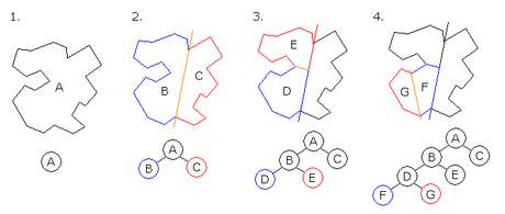
Fig.1. 1 A BSP-tree example [5]
PROBLEM STATEMENTS
Modern day graphical computational demands are complex and computation costs are high. Even the powerful GPUs can’t give best performance if the whole computation is done at same time. But if computation takes place piecewise i.e. on some portions which are active at that period, the GPU’s performance may give the best results because the powerful GPU is now working for only the small portion that means less load hence more efficiency. Now for piecewise computation
How to render a set of opaque or partially transparent objects in 3D-2D space quickly in a visually realistic way is a fundamental problem in computer graphics .A central component of this problem is hidden-surface removal : given a set of objects, a viewpoint, and an image plane, compute the scene visible from the viewpoint on the image plane. Due to this problem hidden-surface removal problem has been studied extensively in both computer graphics and computational geometry.
One of the conceptually simplest solutions to this problem is so called Binary Space Partition Algorithm.
Binary Space Partition (BSP) is a data structure that fragments the objects and ensures that a back-to-front order from a given viewpoint for an arbitrary set of objects.
BSP have proven to be versatile, with applications in problems such as –
Global illumination, shadow generation, visibility problem, solid geometry, ray tracing, robotics, and approximation algorithms for network design and surface simplification.
We use queries that are typically made in many BSP-based algorithms:
1. Point location: determine the leaf of the BSP that contains a query point. Point location is the basis of many algorithms for answering other queries.
2. Ray shooting: determine the first rectangle intersected by a query ray. Ray shooting is a very useful query in visibility problems, since it can be used to determine the object visible along a given direction.
3. Line stabbing: compute the number of leaves of the BSP intersected by a query line. This query models the process of tracking the viewpoint in walk-through applications.
Although a BSP is a tree, we will often discuss just how to partition the box represented by a node into two boxes. We will not explicitly detail the associated construction of the actual tree itself, since the construction is straightforward once we specify the cutting plane.
By this approach the piecewise approach is applied.
LITERATURE REVIEW
Study of various research papers on BSP are as follows:
- ON VISIBLE SURFACE GENERATION BY A PRIORI TREE STRUCTURES
Henry Fuchs, M. Kedem and Bruce F. Naylor in [1] concluded an algorithm to resolve the problem of hidden surface and rapid generation of 3-D realistic images in their research. As many interfaces/applications has their environment consisting of polygons with static geometric relations only the viewing-position is changing so static things can be preprocessed to reduce the run-time computations. They framed this preprocessing to generation of “Binary Space Partitioning” tree, whose inorder traversal would give the polygons in visibility priority.
The problem stated to be solved in their research was to generate a colored image of the environment same as it appear from a viewing position. According to them this image generation consists of 3 steps:-
- Creating points into the image space.
- Clipping all the polygons which lie outside the field of sight.
- The remaining polygons contribute to generation of image. The image consists of color for each, approximate 2,50,000 (500 rows with 500 in each row) pixels. For each pixel
- Closest (Visible) polygon to the viewing position is found.
- Proper color for the pixel of closest polygon is determined.
Now for the above mentioned problems, they proposed solution in which the first 2 steps can be performed easily. They concentrate more on solution for step 3, in that also more specifically on part (i). For several applications, the generated images are of same environment, the only change is in viewing position. E.g. In flight simulation pilots may practice different landings at same airport, where each landing generates many new images. Thus taking advantage of such environments, the database is preprocessed and transformed into BSP tree which at the time of image generation yield a visibility priority value for each polygon[1]. These priorities values are allocated in a way that at each pixel, the polygon closest to the viewing position is given highest priority and remain same for every pixel in image formed from same viewing position. Sometimes priorities values cannot be allocated to original polygons because they need to be split. This splitting is done only during preprocessing.
The proposed solution seems to be more efficient than other previous solutions, for the above mentioned cases. Weakness- A situation with increase in number of original polygons in database with respect to the number in BSP tree has not encountered.
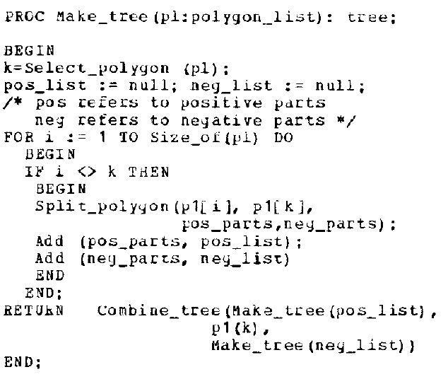
Fig. 2. 1 Tree making process [1]
- PREDETERMINING VISIBLITY PRIORITY IN 3-D SCENES
The calculations performed by many (almost all) visible surface algorithms returns the visible polygon at each pixel in the image. Many researches have been done on the same problem to reduce complexity as well as improve efficiency, but by taking advantage of an observation that without knowing the viewing position and orientation visibility calculations can be performed. The basis of the model is potential obstruction relation between polygons in environment. The method was applicable for only certain objects.
The research provides solution to the above problem which allows determination forall objects according to visibility priority without any manual involvement. H. Fuchs, Zvi M. Kedem and Bruce Naylor also mentioned about the development of stronger solutions, using which these visibility calculations can be reduced. This reduction may lead to significant reduction in processing and memory requirements.
The priority faced within a cluster can be computed independent to viewpoint. For a given figure if, we eliminate the back faces for any viewpoint and assign numbers to the remaining faces then the assigned numbers are the priority numbers. A cluster is a collection of faces that can be assigned a fixed set of priority numbers which after back edges are removed, provide correct priority from any viewpoint.[4]
Face priority computations computes that whether face A (let say) hide face B from any viewpoint. These computations are applied to all faces of the cluster through which a priority graph can be created which can be used to update the priorities dynamically. If any loop exists in graph then the faces cannot be assigned priorities, in that case the cluster needed to be split into smaller clusters.
The researchers proposed a conclusion that:-
Let R= {r1, r2… rn} be a cluster of (convex) polygons which may be considered as describing individual object or entire scene of objects. According to the function f:Z+ , Z+ ={ 1.2….}[2] if both riand rjare visible from outside the object and if riand rj are both facing towards the viewer , then f(ri) <= f(rj) if and only if rj cannot obstruct ri. Now for any point P outside the object, if a ray from P intersects both riand rj and both ri, rjface P, then riobscures rj provided that
f(ri) < f(rj).
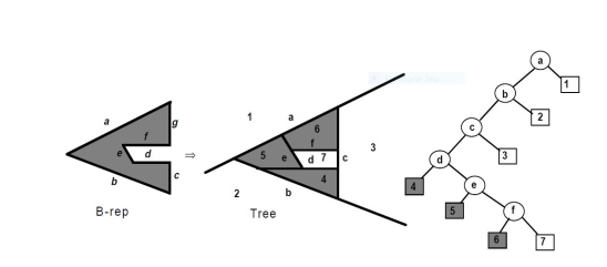
Fig. 2. 2 B-Rep and Tree representation of polygon [6]
- OPTIMIZATION OF THE BINARY SPACE PARTITION ALGORITHM (BSP) FOR THE VISUALIZATION OF DYNAMIC SCENES
Initially developed Binary Space Partitioning algorithms provide an efficient method for visualization of static environment scenes in order to solve Visible Surface Determination problem.
This research describes advancements in generation of BSP trees and its utilization in the visualization of dynamic polyhedral scenes[3]. A new six-level tree structure named as dynamic BSP trees are presented. These trees depend on the incorporation of five various types of auxiliary planes in the creation of BSP trees. Before any scene of polygons these planes are added in the structure. In most of the cases addition of polygons is performed in 0 time by using precomputed BSP trees for single objects.
Dynamic BSP trees results in reduction of computation time used to create BSP tree and its utilization for complex scenes at interactive speeds where viewport and objects, both are dynamic.
The researchers proposed some conclusions:-
- When an object is moved, the plane representing the object must be removed and re-inserted.
- For simplification only static geometry must be inserted into BSP tree.
KEY CONCEPTS
BSPnode: BSPnode is the primary data structure in the algorithm. A node can be referred to as the encapsulation of data- in this case, the 4 coordinates of the area it encapsulates and its 2 children nodes. It is the basic individual point of data in a data set or network, in this case the set being a tree. A single BSPnode is part of the final BSP tree, that can be used to show and represent a region, as well as the link to other nodes. The node has the following main compartments
- 4 variables to store the region: The primary use of the node is to store the data of the region it represents, called ‘x’, ‘y’, ‘h’, ‘w’.
- ‘x’ indicates the base x-axis value of one node. It marks the minimum value of x-axis for the region.
- ‘y’ indicates the base y-axis value of one node. It marks the minimum value of y-axis for the region
- ‘h’ indicates the height of the region covered. It marks the maximum value of y-axis for the region
- ‘w’ indicates the width of the region covered. It marks the maximum value of x-axis for the region.
- 2 address allocators: to store the address of the front and back sub trees to the current node, called front and back.
- ‘front’ indicates the forward half of the tree. The forward sub tree will give the partition in the forward half, meaning that it stores further partitions in the front region.
- ‘back’ indicates the backward half of the tree. The backward sub tree will give the partition in the back half, meaning that it stores further partitions in the back region.
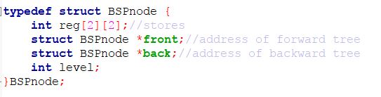
Fig. 3.1 Code snippet of BSPnode
BSPtree: The final tree obtained at the end of the entire algorithm is the BSPtree. It has various properties
- It is created only once.
- The tree arrangement is such that each node may either have no children, or 2 children. Children with one node are not possible.
- The tree is balanced, meaning it forms a perfect triangle shape. If one node has children at the lowest level, it means that its siblings will also have children at that level.
- The leaf nodes of a BSP tree indicate the areas and the break-ups of the region, such that if we want to see the partitions in the region, only the leaves need be shown.
- The tree is used to dynamically find the player location.
- This algorithm, coupled with a rendering method or algorithm, like the painter’s algorithm, is used to dynamically render objects around a camera viewport.
- Traversal within the tree is done without much complexity overhead, and new nodes and regions can be created with ease.
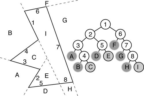
Fig. 3.2 A Complex BSP [7]
MODEL
BSP and BSP-tree are made by recursive subdivision of base region till the satisfactory number of subparts are reached.
- Case 1. Number of Iteration: 0
Region:

Fig. 4.1
BSP-tree:
A
Explanation: When no iterations take place, the tree is only the root node, with no front or back tree. The root node is the representation of the entirety of the region of the map.
- Case 2. Number of iterations: 1
Region
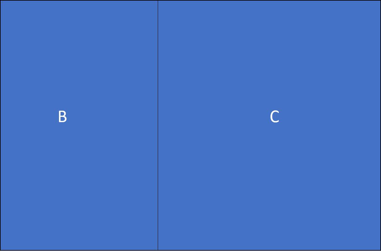
Fig. 4.2
BSP-tree
A


B
C
Explanation: When one iteration is performed, the tree starts branching. The main region is now split between 2 regions.
- Case 3. Number of iterations: 2
Region
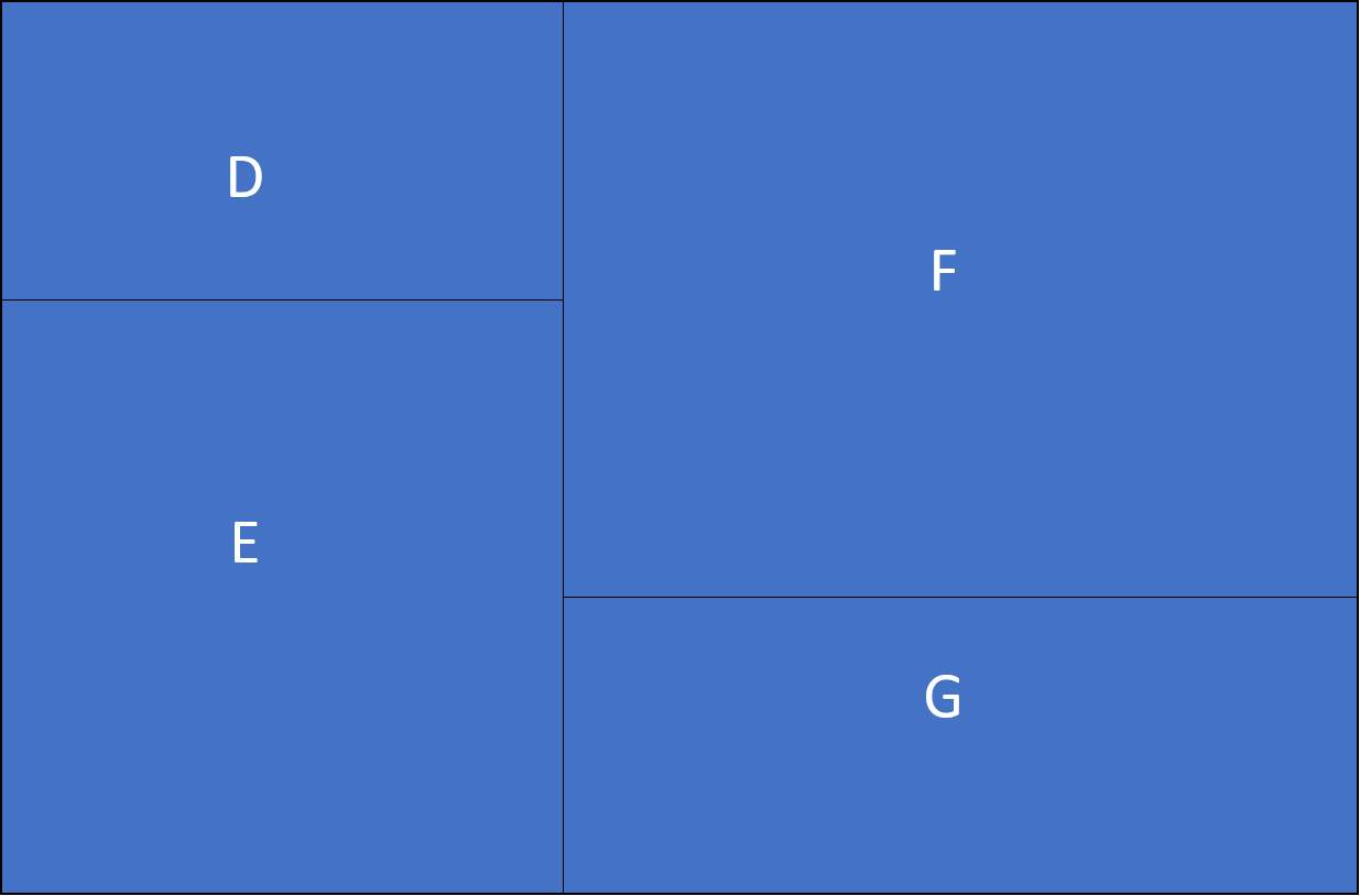
Fig. 4.3
BSP-tree
A


B
C
D
E
F
G
Explanation: When 2 iterations have happened, 4 nodes appear. They populate 4 regions in the map
- Case 4. Number of iterations: 3
Region
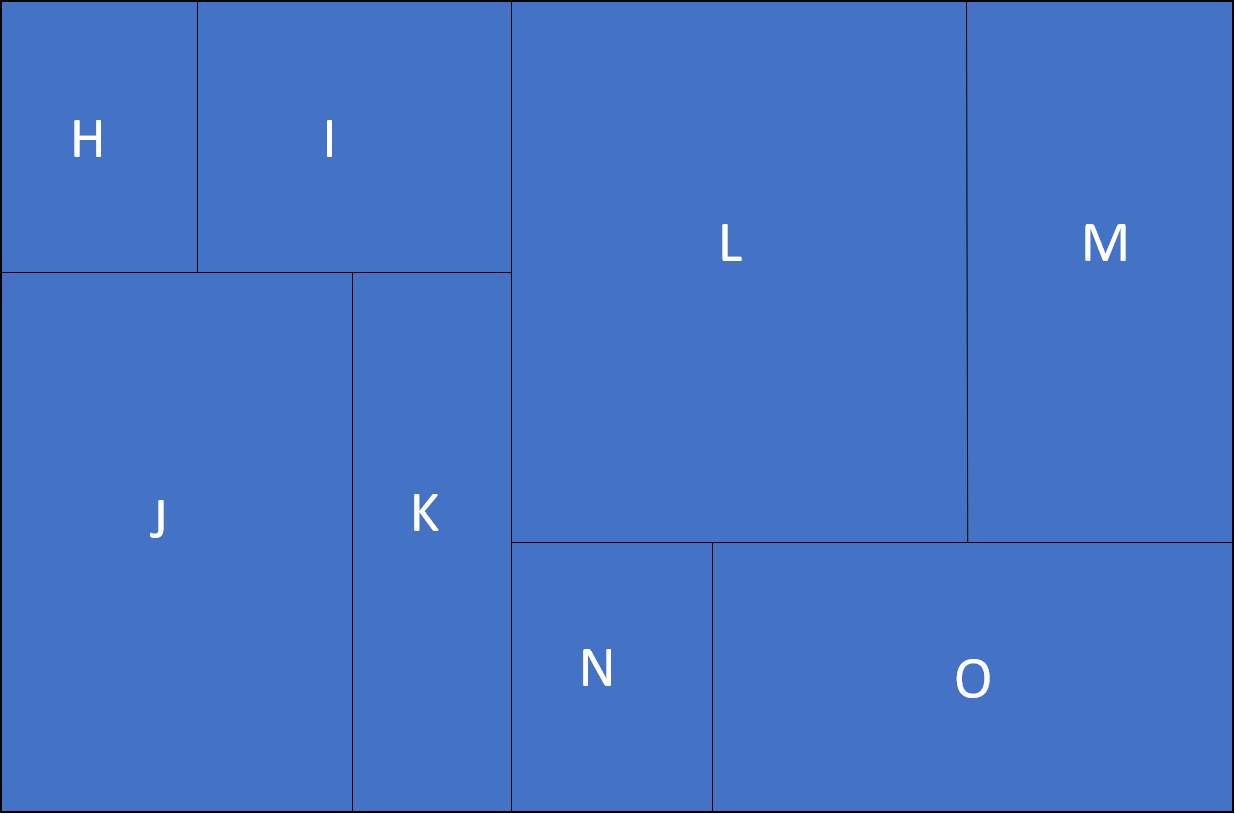
Fig. 4.4
BSP-tree
A


C
B
F
E
D
G
O
N
M
L
K
J
I
H
- Case repeated until required objective is attained.
ALGORITHM
- Split(): Split function is the primary function of the algorithm. Its task is to convert one region into 2 smaller regions. It has the following compartments:
Input: BSPnode ‘a’ – a node of the BSP tree that encapsulates the region. Address allocators front and back initially have no values.
Output: BSPnode ‘b’ and ‘c’- two nodes of the BSP tree, encapsulating 2 regions. Sum of these 2 regions is the region of ‘a’. After the algorithm has executed, ‘a’ will have 2 values in the address allocators. Back of ‘a’ is ‘b’ and front of ‘a’ is ‘c’.
Line by line breakdown of the algorithm.
- BSPnode b, c
This statement creates 2 data structures of BSPnode type, defined as above. These regions will be formed from the one combined region, received as input.
- Allocations:
- b.back = NULL;
- b.front = NULL;
- c.back = NULL;
- c.front = NULL;
This statement allocates the address allocators to default (null) value.
- if (random(0, 1) == 0) {
This statement chooses a random number between 0 and 1, and decides the split accordingly. If random number is 0, the division is done vertically. If the number is 1, division is done horizontally. The following path follows the vertical division.
- b = new BSPnode(a.x, a.y, random(1, a.w),a.h);
This statement assigns values as follows
- b.x=a.x
- b.y=a.y
- b.w=random(1,a.w)
- b.h=a.h
‘b’ node gets a new region. This region is taken from ‘a’ node, such that it retains the minimum ‘x’ and ‘y’ values and even the maximum ‘y’ value. The random function is the important function here. It allocates a random value of ‘x’. This adds a ‘random’ nature to the algorithm, just like real regions.
- c = new BSPnode(a.x + b.w, a.y, a.w – b.w, a.h);
This statement assigns values as follows
- c.x=a.x+b.w
- c.y=a.y
- c.w=a.w-b.w
- c.h=a.h
‘c’ node gets a new region. This region is taken from ‘a’ node, such that it retains maximum values of ‘x’ and ‘y’ values, and even minimum ‘y’ value. The minimum ‘x’ value is computed as the remaining region from the ‘a’ node not occupied by the ‘b’ node.
- if (DISCARD_BY_RATIO) {
This statement regards the ratio. A preestablished base ratio is assumed. If the randomly generated number yields a ratio less than that of the base assumed ratio, we can discard that value, and then find new value and repeat the previous steps to find a ratio that suits the need of the algorithm.
- varb_w_ratio = b.w / b.h
This statement calculates the ratio of width to height for the specific node ‘b’. This is stored in a variable ratio.
- varc_w_ratio = c.w / c.h
This statement calculates the ratio of width to height for the specific node ‘b’. This is stored in a variable ratio.
- if (b_w_ratio< W_RATIO || c_w_ratio< W_RATIO) {
This statement compares the said ratios to the base assumed ratio. If the ratios fail in either of the conditions, said ratio is to be discarded, and function is called again.
- return random_split(BSPnode)}
This statement calls the function again.
- else {
This statement goes to the alternative path where division is done horizontally.
- b = new BSPnode(a.x, a.y, a.w, random(1, a.h)
This statement assigns values to the node as follows:
- b.x=a.x
- b.y=a.y
- b.w=a.w
- b.h=random(1, a.h)
‘b’ node gets a new region. This region is taken from ‘a’ node, such that it retains the minimum ‘x’ and ‘y’ values and even the maximum ‘x’ value. The random function is the important function here. It allocates a random value of ‘y’. This adds a ‘random’ nature to the algorithm, just like real regions.
- c = new BSPnode(a.x, a.y + b.h, a.w, a.h – b.h)
This statement assigns values to the node as follows:
- c.x=a.x+b.w
- c.y=a.y
- c.w=a.w-b.w
- c.h=a.h
‘c’ node gets a new region. This region is taken from ‘a’ node, such that it retains maximum values of ‘x’ and ‘y’ values, and even minimum ‘x’ value. The minimum ‘y’ value is computed as the remaining region from the ‘a’ node not occupied by the ‘b’ node.
- if (DISCARD_BY_RATIO) {
This statement regards the ratio. A preestablished base ratio is assumed. If the randomly generated number yields a ratio less than that of the base assumed ratio, we can discard that value, and then find new value and repeat the previous steps to find a ratio that suits the need of the algorithm.
- varb_h_ratio = b.h / b.w
This statement calculates the ratio of height to width for the specific node ‘b’. This is stored in a variable ratio.
- varc_h_ratio = c.h / c.w
This statement calculates the ratio of height to width for the specific node ‘b’. This is stored in a variable ratio.
- if (b_h_ratio< H_RATIO || c_h_ratio< H_RATIO) {
This statement compares the said ratios to the base assumed ratio. If the ratios fail in either of the conditions, said ratio is to be discarded, and function is called again.
- return random_split(BSPnode)}}}
This statement calls function again.
- return [b, c]
This statement returns 2 new nodes ‘b’ and ‘c’. The split, at the end of the algorithm is such that
a = ∑(b,c)
Summation of the coordinates of region of ‘b’ and ‘c’ gives the coordinates of region of ‘a’.
- Recursive Split: Recursive Split is the control function of the algorithm. It splits the region recursively into partitioned subtrees, till the level required.
Input: BSPnode* region and leaf of partitioning
Output: Recursively partitioned subtree, till a particular tree level
Line by line breakdown:
- If(level > iteration)
This statement is the limiter of the algorithm. ‘Iteration’ is predefined at the start of the entire algorithm. Number of iterations is the number of times that this function is called. One iteration creates 2 splits for each region. This happens as follows
- Iteration=0, splits=0
- Iteration=1, splits=1
- Iteration=2, splits=2
- Iteration=3, splits=4
- Iteration=n, split=2n
As is clear, for ‘n’ iterations, 2n splits are called. This leads to the final complexity being 2n for the split function.
- Return;
This statement marks the end of the algorithm.
- Region.level=level
This statement adds a new level, telling the algorithm to proceed accordingly.
- split(region)
Split function is called from this, leading to formation of new nodes for the tree and new regions for the map.
- Recursive split( region.back, level+1)
Recursive split is called for the back half of the map with respect to the node.
- Recursive split( region.front, level+1)
Recursive split is called for the front half of the node and the map.
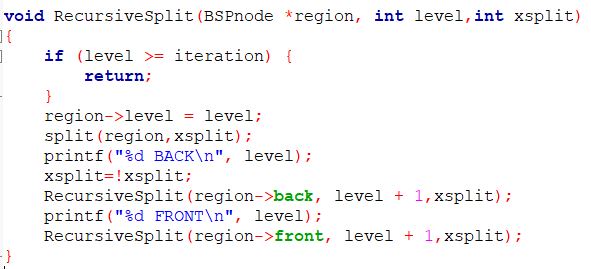
Fig. 5. 1. Snippet of The recursive split function
RESULT AND DISCUSSION
- Problems
Identifying portions of a scene, object or a game map that are visible from a position chosen for viewing is major area of concern for the generation of realistic graphic objects in games, rendered images and animations. Issues such as window-to-viewport transformation and mapping, framerates, polygon count and shading combine to give multiple problems relating to rendering.
To resolve the problem various approaches are devised, and correspondingly multiple algorithms are made for identification of visible objects efficiently which may vary for different types of application areas.
The methodology also varies depending upon the criteria or situation such as some require large amount of memory, so takes more time to process the data set, and some which are only applicable on a specific special type of objects.
The decision parameter for choosing a method depends on many factors such as the scene or map complexity, type of game object which must be showcased, all the possible and available equipment’s, also whether the displays are to be generated are static or have motion involved.
These set of various algorithms or approaches are referred to as Visible Surface Detection methods or, conversely as Hidden Surface Elimination methods. Such methods become paramount when you take into account the present day graphically intense Computer-Generated Images(CGI) involved in the entertainment industry. The algorithms, although appearing rudimentary in nature, provide extensive utility in the present-day scenario.
These steps become essential when we factor the variety of computers, game consoles and mobile phones available to the consumer in the present day. This is a booming industry, and every developer, artist or art designer, who intends to provide various consumers with a similar experience of their product, different specifications can lead to varying performances and issues across mediums. Avoiding these obstacles needs careful understanding and deep research of rendering algorithms.
- Variations and methods
Depending upon whether the specific algorithm or approach deals with object definitions directly or their images which are projected, these algorithms are mainly classified into two types which are:
- Object-Space methods
- Image-Space methods
In an Object-Space methodology within the scene or map definition each object is checked for visibility, and labelled accordingly, which makes a comparison of objects and other parts of objects. It is, therefore, implemented in physical coordinate system. It is continuous in nature. More accurate, but more complex, computationally
In an Image-Space methodology at each position of the pixel on the plane of projection the visibility of objects is decided point by point, and is implemented on the screen coordinate system unlike object-space method. Discrete in nature. Less detailed, so lower complexity.
In general, both the approaches use sorting and coherence techniques to enhance the performance of the results.
Sorting by ordering the individual surfaces in a scene are used to facilitate comparison of the depth of the object to their distance from the plane of viewing.
In general, both the approaches use sorting and coherence techniques to enhance the performance of the results.
Sorting by ordering the individual surfaces in a scene are used to facilitate comparison of the depth of the object to their distance from the plane of viewing.
These algorithms work on the concept of coherence and its properties. These properties aid these algorithms in avoiding unnecessary calculations. Coherence is created by local similarity.
Properties/Types of Coherence:
- Object Coherence
Whenever an object is completely different from another, has a unique data set then we do not need to compare them anymore.
- Face Coherence
Whenever we observe a smooth and a constant variation across a face what we need to do is incrementally and gradually modify.
- Edge Coherence
We always need to remember that the visibility of the objects changes whenever an edge crosses behind a face that is visible.
- Implied Edge Coherence
A line that is a line of intersection of a face planar and penetrating another can be obtained easily from the two-point plotted on the intersection.
- Scanline Coherence
Remember that the successive lines always have a similar type of span.
- Area Coherence
The span of pixels which are of adjacent groups are often covered by the faces that are visible.
- Depth Coherence
We must use the difference equations which estimates the actual depth of all the nearby points on the same surface.
- Frame Coherence
Two successive frames in an animation sequence may be similar, employing only minor changes in viewpoint and objects.
Each of the Hidden Surface Removal methods is with its own set of strengths and weaknesses. Alternate methods for the rendering with hidden surface removal, besides BSP, are:
- Detecting the Back-Faces
- Back Face detection is Object-space method.
- Back-Face detection method involves vectors and identifying if a point lies inside a polygon surface or outside.
- The algorithm relies on viewing vector and normal vector of objects. An object will be a back face if the Dot Product of the two vectors is greater than zero, i.e. V.N>0
- Advantages
- Relatively simple calculation.
- May even eliminate up to 50% surfaces, making it faster.
- Disadvantages
- Partially hidden surfaces cannot be determined.
- Other operations like raytracing cannot be performed.
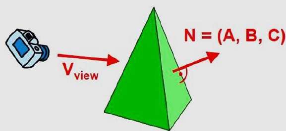
Fig. 6. 1 Back- Face detection. [8]
- Method of Depth or Z-Buffer
- Z-buffer is an Image space approach.
- The general algorithm determines the nearest visible surface to the camera perspective.
- The algorithm starts by searching for the surface pixels with the lowest values of Z-buffer. As the surface is drawn this value is adjusted and the algorithm proceeds to the next lowest value, until infinity is reached. The algorithm maintains 2 data structures
- Depth buffer (Z-buffer)
- Refresh buffer (intensity buffer)
- Advantages
- The algorithm is relatively easy to implement.
- Speed complexity is low, if programmed on hardware.
- It processes one object at a time.
- Disadvantages
- Space complexity is high.
- Time consuming process.
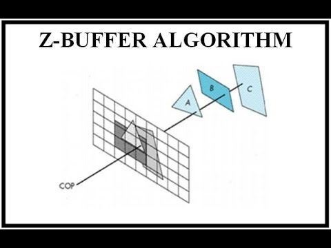
Fig. 6. 2 Z-Buffer or Depth Buffer algorithm [8]
- Method of Scanline
- Scanline method is an image space approach.
- Also referred to scanline Z-buffer, as it is a Variation of the Z-buffer algorithm.
- Depth information for a single scan line is provided by this algorithm.
- Each new scan line provides a new value, and re-initializes the algorithm.
- Two separate tables are created for this algorithm to work
- Edge Table
- Polygon Table
- Advantages
- Compared to the basic Z-buffer, this method requires far less memory.
- Disadvantages
- Time complexity is still high.
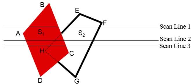
Fig. 6. 3 Scanline Algorithm [8]
- Method of depth sorting
- Depth sorting is also called Painter’s Algorithm.
- It takes its name from the techniques painters apply, where they paint the background first and draw the closer regions later.
- The painter’s algorithm arranges all polygons in 3D space to be converted to 2D based on the distance from the screen. Rendering then happens from the farthest region to the nearest.
- This algorithm’s solution to hidden surface problem is to paint over said regions. In drawing from far to near, areas to be hidden are eventually drawn over. This comes at the expense of overdrawing.
- Every wall, every object and everything is rendered.
- Advantages
- Once rendered, objects need not be rendered again, so this is easier to work with.
- Other methods work with depth sorting to allow better rendering. BSP with Painter’s algorithm is one example.
- Disadvantages
- Overdrawing takes place extensively.
- Very resource expensive.
- Cyclic overlapping or piercing polygons cannot be drawn in this way.
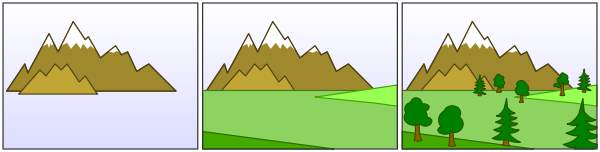
Fig. 6. 4 Idea of Painter’s algorithm[8]
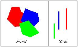
Fig. 6. 5 Painter’s algorithm rendering [9]
- Method of octrees
- Octree is a tree data structure where every internal node has 8 child nodes.
- They are used to partition a 3D space by recursively subdividing it into child nodes.
- Traversed using DFS (Depth First Search)
- 3×3 matrix is also used for representation.
- Advantages
- Access time is low.
- Disadvantages
- A lot of nodes are generated for few objects.
- Geometry management may become very complex.
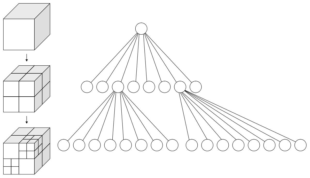
Fig. 6. 6 Octrees[8]
- Method of A-Buffer
- Form of image space order.
- Also called anti-aliased buffer, or area averaged buffer or accumulation buffer.
- Resolves issues such as partial visibility- transparent, translucent and opaque objects can be made.
- It also accounts for intersecting surfaces.
- Derivative of Z-buffer algorithm.
- Advantages
- Accounts for partial visibility as well as intersection.
- Disadvantages
- Time complexity increases when compared to Z-buffer.
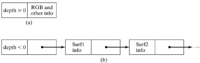
Fig. 6. 7 A buffer algorithm.[10]
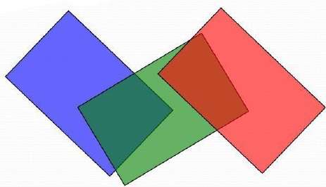
Fig. 6. 8 A-Buffer[8]
- Method of ray-casting
- It is an image-space ordered algorithm.
- Provides multiple solutions for 3D graphics- hidden surface removal and ray tracing for 2D images from 3D scenes.
- Calculations of colours and images done with each pixel.
- Advantages
- No recursion involved, so complexity is very low.
- High speed calculations
- Disadvantages
- Possibility of accurate shadows, reflections and refractions is removed. However, it may be faked to a degree.
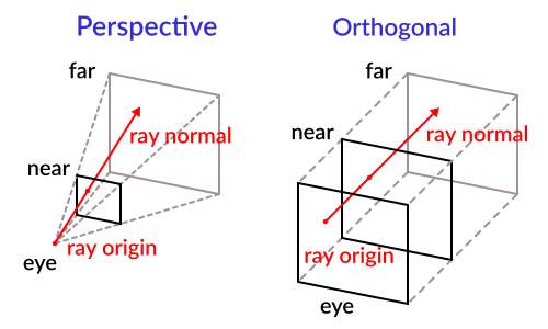
Fig. 6. 9 Ray-casting in perspective and orthogonal view.[11]
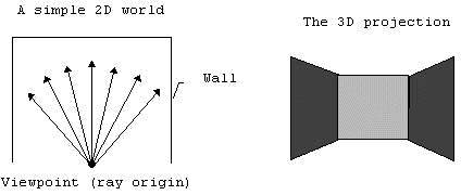
Fig. 6. 10 2D to 3D projection or Ray-casting [12]
- Results
Binary Space Partitioning is used extensively in 3D renders, video games, augmented reality, virtual reality, animation movies, and just about all computer graphics. It’s a relatively simple solution to a complex problem with requiring less resources than its competitors.
The usefulness of the BSP method comes into notice when we view all the references of points that are to be changed, but what matters more is the objects that are in the scene also the positions of all these objects are fixed at a specified position.
Binary space partitioning enables a lot of features that others don’t.
- No overdrawing.
- Complexity of O(2n) is involved when a tree is formed, but this is a one-time cost paid when drawing the BSPtree. Later, traversal of binary tree takes place, which is less expensive O(nlog2n).
- Tree created once is reusable.
- Can be used both in 2D and 3D graphics.
- Identification of all the possible surfaces that actually are the cases which we had discussed earlier of inside/ front, outside/back with respect to the plane of partitioning at each and every step involved in the division of the spaces which are actually relative to the direction of viewing.
- We should always start randomly with a plane and then keep on finding only that one set of objects that are behind, and all the other are in the front.
- The objects or the game elements in the partitioning tree are represented as the nodes which are the terminal ones with objects that are in the front are kept as branches that are on the left and for objects that are at the back are kept on the branches towards the right.
- The root node of a BSP Tree is a polygon which by some parameters are selected on the basis that they are to be displayed.
CONCLUSION
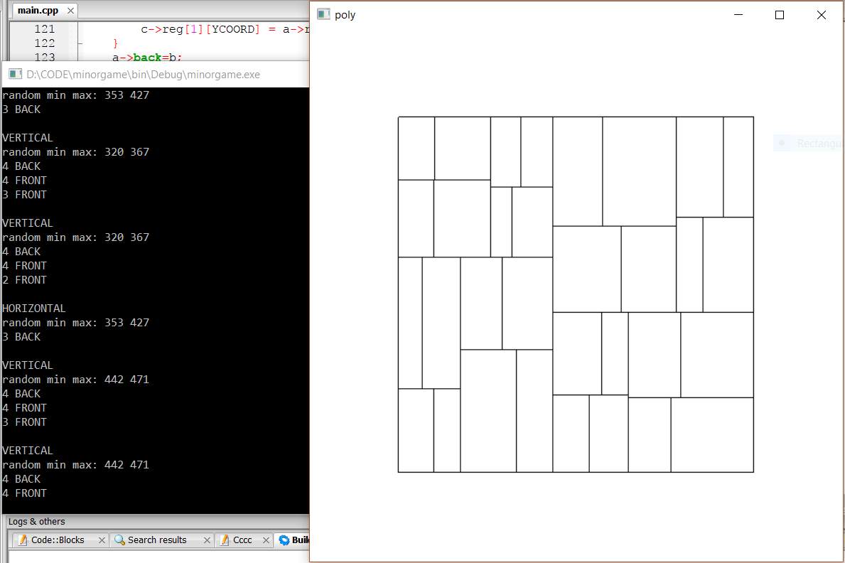
Fig. 7. 1 Output snippet of code for Binary Space Partitioning
BSP and BSP-tree are the industry standards for various kinds of video games and animations. Most, if not all, studios inherently use tools and softwares that implement BSP because of the many advantages that BSP provides- resource conservation, reusability and reliability.
BSP offers better compatiability than other methods as well.
REFERENCES
[1] H. Fuchs, Z. M. Kedem, and B. F. Naylor. On visible surface generation by a priori tree structures. Computer Graphics (SIGGRAPH ’80 Proceedings), 14(3):124{133, July 1980.
[2] [Schumaker et al 69] R. A. Schumackcr, R. Brand, M. Gilliland, and W. Sharp, “Study for Applying Computer-Generated lmages to Visual Sirnulation,” AFHRL-TR-69-14, U.S. Air Force Human Resourccs Laboratory (1969).
[3] Torres, Enric. OPTIMIZATION OF THE BINARY SPACE PARTITION ALGORITHM (BSP) FOR THE VISUALIZATION OF DYNAMIC SCENES, Computer Graphics, 1990.
[4] H. Fuchs, Z. M. Kedem, and B. F. Naylor. PREDETERMINING VISIBLITY PRIORITY IN 3-D SCENES, Computer Graphics, 1980.
[5] Figure 1.1 source:commons.wikimedia.org
[6] Figure 2.2 source: www.cs.princeton.edu
[7] Figure 3.2 source: www.unrealtexture.com
[8]Figure 6.1, 6.2, 6.3, 6.4, 6.6, 6.7, 6.8 source: www.tutorialspoint.com
[9] Figure 6.5 source: www.cs.helsinki.fi
[10] Figure 6.9 source: Godot engine docs
[11] Figure 6.10 source: permadi.com
Cite This Work
To export a reference to this article please select a referencing stye below:
Related Services
View all


Related Content
All TagsContent relating to: "Computer Science"
Computer science is the study of computer systems, computing technologies, data, data structures and algorithms. Computer science provides essential skills and knowledge for a wide range of computing and computer-related professions.
Related Articles

DMCA / Removal Request
If you are the original writer of this dissertation and no longer wish to have your work published on the UKDiss.com website then please: