Experimental Investigation of Fracture Energy of Normal-strength and High-strength Concrete

Abstract

The aim of this report is to investigate the fracture energy of normal and high strength concrete. Concrete is a composite material, a typical concrete mix will contain aggregate, cement & water – although frequently other additives are added to achieve the desired mechanical properties. As concrete is nonhomogeneous, when stressed it cracks due to the different mechanical properties of the constituent materials. The fracture energy is defined as the energy required to open a unit area of crack surface. The understanding of fracture energy is vitally important, as the energy required to crack a concrete sample will vary depending on the mix of the concrete.  The experimental investigations are designed to allow analysis and comparisons of two concrete mixes, C30 and C70 concrete to determine the effects of concrete strength on fracture energy.

Contents

Click to expand Contents

1 Introduction

2 Mix Design

2.1 C30 Mix Design

2.1.1 Stage 1

2.1.2 Stage 2

2.1.3 Stage 3

2.1.4 Stage 4

2.1.5 Stage 5

2.1.6 Final Mix Proportions

2.2 C70 Mix Design

3 Mixing and Sampling

3.1 Concrete Mixing

3.2 Workability

3.3 Curing

4 Testing of Hardened Concrete

4.1 Pundit Test – Ultrasonic Pulse Velocity Test

4.2 Density Test

4.3 Dynamic Modulus of Elasticity

4.4 Schmidt Hammer Test

4.5 Compressive Strength Test

4.5.1 Analysis of Results

4.6 Tensile Splitting Test

4.6.1 Analysis of Results

4.7 Flexural Strength Test

4.7.1 Analysis of Results

4.8 Fracture Energy

4.8.1 Analysis of Results

5 Brittleness

5.1 Bache Method

5.2 Characteristic Length

5.3 Analysis of Results

5.4 Critical Intensity Factor (Fracture Toughness)

5.4.1 Analysis of Results

6 Conclusion

7 Bibliography

Figures

Figure 1 – Flow Chart Design (Building Establishment Research, 1997)

Figure 2 – Standard Deviation (Building Establishment Research, 1997)

Figure 3 – Relationship between standard deviation and characteristic strength (Building Establishment Research, 1997)

Figure 4 – Approximate compressive strength (Building Establishment Research, 1997)

Figure 5 – Relationship between compressive strength and free water/cement ratio (Building Establishment Research, 1997)

Figure 6 – Approximate free-water contents (Building Establishment Research, 1997)

Figure 7 – Estimated wet density of fully compacted concrete (Building Establishment Research, 1997)

Figure 8 – Recommended proportions of fine aggregate according to percentage passing a 600 µm sieve (Building Establishment Research, 1997)

Figure 9 – Types of Slump (Online Civil Engineering, 2010)

Figure 10 – UPV Test (transmission directions)

Figure 11 – C30 and C70 Pundit test results

Figure 12 – Compressive strength and tensile splitting test machine

Figure 13 – Failure conditions of compressive strength test

Figure 14 – C30 & C70 Compressive Strength Test Results

Figure 15 – Typical strength gain curve (Camp, 2017)

Figure 16 – Tensile Splitting Test

Figure 17 – C30 and C70 Tensile Strength

Figure 18 – Table 3.1 from EC2

Figure 19 – C30 and C70 flexure strength

Figure 20 – Crack modes (Dascalu, 2011)

Figure 21 – Three-point bending test

Figure 22 – Three-point bending test machine Figure 23 – Three-point bending test apparatus

Figure 24 – Fracture Process Zone (Gdoutos, 2005)

Figure 25 – Typical load/displacement curve

Figure 26 – C30 Vs C70 – Load/Displacement

Tables

Table 1 – C30 Mix Design Specified or Known Values

Table 2 – C30 Mix Proportions (1m3)

Table 3 – C70 mix proportions (1m3)

Table 4 – C30 and C70 final trial mix proportions

Table 5 – Relationship between velocity and concrete quality

Table 6 – Density values of test specimens

Table 7 – C30 and C70 average volumes and density values

Table 8 – Dynamic modulus of elasticity

Table 9 – C30 and C70 compressive strength test results

Table 10 – C30 & C70 Tensile Strength

Table 11 – C30 and C70 flexure Strength

Table 12 – Fracture energy standard parameters

Table 13 – C30 and C70 fracture energy results

Table 14 – C30 and C70 brittleness index

Table 15 – C30 and C70 Elastic modulus

Table 16 – C30 and C70 characteristic length

Table 17 – C30 and C70 Fracture toughness

Appendix A – C30 & C70 Design Mix

Appendix B – C30 & C70 Load Vs Displacement Graphs

1 Introduction

An attempt has been made in this report to compare the differences in fracture energy of both normal and high strength concrete. To investigate these differences, two test mixes have been designed, mixed, and cured under laboratory conditions to create adequate test specimens to allow both non-destructive and non-destructive for data analysis. A total of 4 cubes and 3 beams have been tested for each concrete mix which comprises of a C30 and C70 mix.  The report will provide analysis of the results, with attention given to the destructive tests to aid discussions on the noted differences in calculated fracture energy of the mixes.

2 Mix Design

To complete the required laboratory testing, samples will be required of both normal and high strength concrete mixes. To facilitate this, two mix design will be completed, one for C30(30Mpa) and C70 (70mpa). To allow for better comparison of results, both mixes will be made from the same constituent materials, although the quantities of these materials will change as required by the prescribed characteristic strength. The constituent materials are as follows;

• Ordinary Portland Cement (OPC) class 52.5N
• 20mm granite for coarse aggregate
• Crushed granite for fine aggregate
• Tap water (suitable for drinking)

The mix design of both mixes is based on the flow chart procedure in accordance with Figure 1.

Figure 1 – Flow Chart Design (Building Establishment Research, 1997)

The procedure is split into 5 stages, with each stage responsible for an aspect of the mix design. The stages are as follows:

Stage 1 – deals with strength leading to the free-water/ cement ratio

Stage 2 – deals with workability leading to the free-water content

Stage 3 – combines the results of Stages 1 and 2 to give the cement content

Stage 4 – deals with the determination of the total aggregate content

Stage 5 – deals with the selection of the fine and coarse aggregate contents

The flow chart begins with specified values on the left and ends with either a mix parameter or a unit proportion on the right, depending on which stage is being considered. The specified values are values specified by the designer and depends on the required strength (stage 1), workability (stage 2) and durability (stage 3). All this information should be detailed within the designer’s structural concrete specification.

2.1 C30 Mix Design

The mix design process requires specified data and known information about the constituent materials to complete the process in accordance with Figure 1. Both the specified and known additional information regarding the C30 mix design is presented in Table 1.

Specified Values
Item	Value	Reference
Characteristic Strength	30 N/mm2	Spec
Cement Strength Class	52.5N	Spec
Slump	30-60mm	Spec
Maximum Aggregate size	20mm	Spec
Percentage of defectives (5%)	1.64
Additional Information
Relative density of aggregate (SSD)	2.57
Aggregate Type	Crushed (granite)

Table 1 – C30 Mix Design Specified or Known Values

2.1.1 Stage 1

Stage 1 deals with the strength of the mix, which ultimately leads to the required free-water / cement ratio.

2.1.1.1 Standard Deviation

Due to concrete being a mix with many variables, it will inevitably experience a range of results, even for the same mix design. This can be due to many reasons, such as; difference in the saturation of the aggregate, inconsistency in cement, mixing etc.  It is generally accepted that the variation in concrete strength follows the normal distribution as shown in Figure 2, where s = Standard deviation.

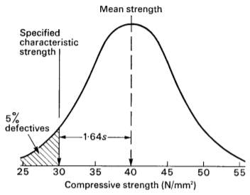
Figure 2 – Standard Deviation (Building Establishment Research, 1997)

The standard deviation is a function of n (number of tests) and is only an estimate. It is therefore subject to normal probability errors which reduce as n increases; therefore S decreases when n increases. The standard deviation can be calculated using the below formula but should only be used when reliable production data is available. In absence of suitable data, Figure 3 should be used. The lab investigations will produce less than 20 results, therefore for characteristic strength of 30 N/mm², the standard deviation is 8 N/mm².

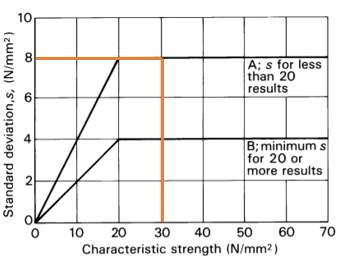
Figure 3 – Relationship between standard deviation and characteristic strength (Building Establishment Research, 1997)

2.1.1.2 Margin and Target Mean Strength

Due to the variation in concrete test results, it is necessary to design the mix for a mean strength greater than the specified characteristic strength. By doing this reduces the risk of a high percentage of failures. However, it is still reasonable to expect a certain level of failures, the control levels to ensure 0% failures is impractical. K is a constant which has been calculated based on normal distribution and is dependent on acceptable percentage of defectives. The below are the derived values of K based on percentage of defectives;

k for 10% defectives = 1.28

k for 5% defectives = 1.64

k for 2.5% defectives = 1.96

k for 1% defectives = 2.3

(Building Establishment Research, 1997)

The product of ks is the margin, which added to the characteristic strength provides the mean strength. Naturally, as the allowed percentage of defectives decreases, k increases as ultimately this increases the margin and the mean strength. Calculating the Margin is based on formula C1 and the mean strength based on C2

C1 = M = k x s

Where;

M = Margin

K = percentage of defectives

S = standard deviation

M = 1.64 x 8

M = 13.12N/mm²

C2 = fm = fc + M

Where;

Fm = the target mean strength

Fc = the specified characteristic strength

M = Margin

Fm = 30 + 13.12

Fm = 43N/mm²

2.1.1.3 Free Water/Cement Ratio

The free water/cement ratio is a vital part of the mix design, it affects the concrete strength, workability and durability. The data from Figure 4 provides the approximate compressive strength of a mix, for a given period, based on a w/c ratio of 0.5, cement class and aggregate type (crushed/uncrushed). This data is used along with the target mean strength of the specified characteristic strength to determine the required water/cement ratio.

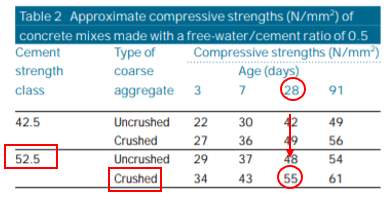
Figure 4 – Approximate compressive strength (Building Establishment Research, 1997)

Based on the known data of the mix, the approximate strength is 55N/mm² in accordance with Figure 4. Using this value, a horizontal line is plotted on Figure 5, and from this point a curve parallel to the printed curves is plotted. A horizontal line is then drawn from the target mean strength until it intersects with the new curve. The intersection point determines the required w/c ratio.

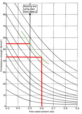
Figure 5 – Relationship between compressive strength and free water/cement ratio (Building Establishment Research, 1997)

Based on Figure 4 and Figure 5, a free water/cement ratio of 0.6 is required. It is clear from the graph that as the required compressive strength increases, the free-water/cement ratio decreases.

2.1.2 Stage 2

Stage 2 deals with workability. The only value to be calculated at stage 2 is the free water content.

2.1.2.1 Free Water Content

Free water includes the water required to achieve an aggregate SSD condition, and the water required for the hydration of the concrete for the specified workability. Calculations are typically based on an SSD condition, which is this is the closest to the actual condition of most aggregates which are stored at a plant.

To determine the free water content reference is made to Figure 6 which provides the required water content in kg for 1 m³ of concrete. The content varies depending on the aggregate size/type and the required workability. Based on our parameters, the required free-water content is 210kg/m³.

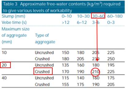
Figure 6 – Approximate free-water contents (Building Establishment Research, 1997)

2.1.3 Stage 3

Stage 3 combines the results of stage 1 and 2 to provide the cement content. After calculating, it may be necessary to increase the content based on the specified minimum cement content. In the case of this experiment, a minimum cement content is not provided. If the cement content is increased from the calculated value, it will be necessary to calculate the modified free-water/cement ratio.

2.1.3.1 Cement Content

Cement content is calculated as shown below (Building Establishment Research, 1997).

Cement content =

3)

C = the cement content (kg/m³)

W = the free water content (kg/m³)

Total aggregate content = 2340 – 350 – 210

Total aggregate content = 1780 kg/m³

2.1.5 Stage 5

Stage 5 is the final stage and is responsible for determining the ratio of the coarse and fine aggregate contents. To calculate requires a knowledge of the grading of the fine aggregate by determining the percentage of fines passing a 600μm sieve.

2.1.5.1 Proportion of Fine Aggregate

The grading of the fine aggregate used in this experiment results in 52% of fines passing a 600μm sieve. Based on this, Figure 8 recommends a 37% proportion of fine aggregate based on a workability requirement of 30-60mm, free water/cement ratio of 0.6 and a maximum aggregate size of 20mm.

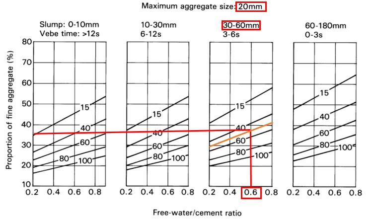
Figure 8 – Recommended proportions of fine aggregate according to percentage passing a 600 µm sieve (Building Establishment Research, 1997)

2.1.5.2 Fine and Coarse Aggregate Contents

The last calculation to complete the mix design is to determine the respective contents of the fine and coarse aggregate contents based on the recommended proportion of fines from Figure 8.

Fine aggregate content   = total aggregate content x proportion of fines

= 1780 x 37%

= 659 kg/m³

Coarse aggregate content = Total aggregate content – fine aggregate content

= 1780 – 659

= 1121 kg/m³

2.1.6 Final Mix Proportions

Below are the tabulated results of the C30 mix design to produce 1m³. The values are rounded to the nearest 5kg.

Quantities per m3	Cement (kg)	Water (kg)	Fine agg. (kg)	Coarse agg. 20mm (kg)
	350	210	660	1125

Table 2 – C30 Mix Proportions (1m³)

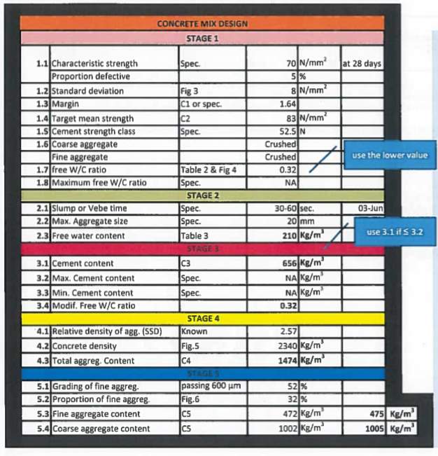
2.2 C70 Mix Design

The C30 mix design section provides, in detail, the approach required to determine the mix proportions for the specified variables. The C70 mix design will follow the same approach, however the specified values will change as the required characteristic strength is now 70N/mm² as opposed to 30N/mm². This procedure will not be replicated again, however the completed design mix form can be found in App A and the required mix proportions have been provided in Table 3.

Quantities per m3	Cement (kg)	Water (kg)	Fine agg. (kg)	Coarse agg. 20mm (kg)
Quantities per m3	656	210	475	1005

Table 3 – C70 mix proportions (1m³)

3 Mixing and Sampling

Production of the test samples will use the mix designs as detailed above for both C30 and C70 mixes. To determine the final quantities for production two adjustments are required;

1. Increase water content to achieved aggregate SSD condition
2. Adjust mix quantities for required production volume

The design mix above assumed an aggregate SSD condition, the aggregate used in this experiment is oven dry condition. Therefore, an allowance is required for the water absorption of the aggregate. In the laboratory, it had been measured that 0.71% by mass of water is required to achieve SSD condition (A). Thus, the dry mass of the aggregate can be calculated by 100/(100+A), with the difference between this and the previously calculated quantities equalling the additional water required.

The test samples will consist of four concrete cubes and three concrete beams. Dimensions are in accordance with BS EN 12390-1 with a cube of 100x100x100mm and beam of 100x100x500mm. Based on the volume and number of samples an actual mix of 0.019m³ is required, however a trial mix of 0.024m³ will be produced to ensure the quantity of concrete is at least 10% greater than required by the test samples in accordance with BS 1881-125:2013 .

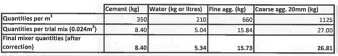
C30 Mix	Cement (kg)	Water (kg)	Fine agg (kg)	Coarse agg 20mm (kg)
Quantities per m3	350	210	660	1125
Quantities per trial mix (0.024m3)	8.40	5.04	15.84	27.00
Final mix (after water content adjustment)	8.40	5.34	15.73	26.81
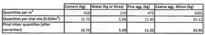
C70 Mix	Cement (kg)	Water (kg)	Fine agg (kg)	Coarse agg 20mm (kg)
Quantities per m3	656	210	475	1005
Quantities per trial mix (0.024m3)	15.75	5.04	11.40	24.12
Final mix (after water content adjustment)	15.75	5.29	11.32	23.95

Table 4 – C30 and C70 final trial mix proportions

3.1 Concrete Mixing

Concrete mixing was completed in accordance with BS 1881-125:2013. The mixing was completed by an industrial mixer and completed as follows;

1. Mixer wiped with damp cloth
2. Aggregate added along with water content required to achieved SSD condition
3. Addition of cement and remaining water

3.2 Workability

Various test can be undertaken to determine the workability of a mix. The slump test is the most common, however a Vebe test can also be completed. If a high workability concrete mix is required, then a flow test may be required. A slump test was used for this experiment with a specified target slump of 30-60mm.

A compliant slump test should be completed in accordance with BS EN 12350-2. A slump test requires the following apparatus;

• Smooth metal cone
• Compacting rod
• Base plate
• Ruler
• Shovel

All of which are to be in accordance with the requirements of BS EN 12350-2.

The test is completed by compacting specified layer thicknesses of concrete into a metal cone. Each layer is to 1/3 of the height of the cone. Compaction should be controlled and completed after placing each layer. A layer requires to be compacted by performing 25 strokes using the compacting rod (BSI, 2000).

Once the sample has been adequately compacted, the cone should be lifted leaving behind the formed concrete cone. Once unsupported by the mould, the concrete will deform under its own self weight creating a ‘slump’. By turning the cone mould on its head, a measurement is taken from the top of the mould to the highest point of the concrete which determines the slump of the mix.

There are four types of slump which are shown in Figure 9. A “true” slump is considered a satisfactory slump test. Both zero and collapsed slumps are out with workability range for a slump test. A shear slump is classed as a failure (BSI, 2000)

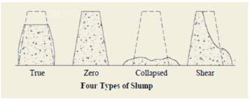
Figure 9 – Types of Slump (Online Civil Engineering, 2010)

The target slump for the mix is 30-60mm. The slump achieved was 140mm and appeared to look like a shear slump. A shear slump typically happens when the concrete is not sufficiently cohesive. Therefore, it could be due to inadequate compacting when creating the slump. In our case, the compaction was provided by a student, and not an experienced technician. For the purpose of our investigation, the concrete was used regardless of the slump test result.

3.3 Curing

Both the C30 and C70 mix were cured under identical conditions. The samples were placed in a water bath at a temperature of (20 +/- 1)° for 7 days and then left in air for 7 days prior to testing. This is different to the recommended procedure in BS EN 12390-2 which states to leave the specimens in water at (20+/-2) ° up until testing (BSI, 2009). The longer concrete is left to cure in water, the greater strength development.

4 Testing of Hardened Concrete

Testing of hardened concrete can be of two forms, destructive testing (DT) or non-destructive testing (NDT). The data required will typically dictate what form is required, however some information could be collected by both forms. When dealing with concrete which is part of an existing structure, it is preferred to complete non-destructive testing (NDT) as these tests will not have an adverse effect on the structure.

As part of the lab experiment, both destructive and non-destructive testing was completed. The same samples were used for both NDT and DT testing. Testing of hardened concrete is governed by BS EN 12390.

4.1 Pundit Test – Ultrasonic Pulse Velocity Test

Pundit test, as it will be referred to herein, is an NDT which should be completed in accordance with BS EN 12504-4. In this experiment, it was used to determine the quality of the concrete samples. The test works by propagating ultrasonic waves through a specimen and records the time taken for the wave to travel. Tests can be completed via direct transmission or indirect transmission Figure 10. Direct transmission is most frequently used and was the method used in the lab experiment.

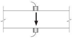
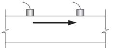
Figure 10 – UPV Test (transmission directions)

By measuring the time taken for the wave to travel, which is constant for an elastic homogenous material, the velocity can be calculated if the distance travelled is known. Although concrete is a strictly a non-homogenous material, at macro level it can be viewed as homogenous.

In principle, a higher velocity should mean the wave has a more direct route between the transducers and therefore highlights small amount of voids indicating good quality. Whereas a low velocity means the route/travel distance has been extended due to void or cracks. The below tables relate velocity to concrete quality

Velocity (km/s)	Quality of Concrete
>4.5	Excellent
3.5 – 4.5	Good
3.0 – 3.5	Doubtful
2.0 – 3.0	Poor
<2.0	Very Poor

Table 5 – Relationship between velocity and concrete quality

Figure 11 presents the results from the pundit test for both the C30 & C70 mix. As can be seen from the results, all tests show the concrete quality to be either good or excellent.

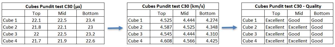
Figure 11 – C30 and C70 Pundit test results

Within Industry, the Pundit test is becoming increasingly used to locate defects in concrete elements of existing infrastructure. In bridges, it is a useful tool in assessing the condition of bridge half joints, which are notoriously difficult to inspect. It can also be used to locate cracks or delaminated concrete. This is possible as the wave is unable to travel across a crack and therefore bounces back. For a concrete element, you can test a sound section to determine the time the wave should take to travel. If the travel time less, it suggests a crack is present. The time taken will also give an idea on the location. (John T. Petro Jr., 2011)

4.2 Density Test

Density is a measurement which relates an objects mass to its volume. For concrete, its mechanical properties are linked to density. A low-density concrete is typically due to voids, for example lightweight concrete is typically created by a high quantity of air entrainment, sometimes referred to as foamed concrete. The voids reduce the concrete density, but also has an adverse effect on its strength. Whereas normal and high-density concrete will have higher density, less voids and increased strength.

Density tests are to be completed in accordance with BS EN 12390-7, the formula for calculating density is below. BS EN 12390-7 provides options for how mass is measured i.e. mass in air or saturated mass and provides guidance for measuring a specimen’s volume.

Density =

massvolume

Equation 1

For this experiment, the volume was calculated by water displacement. However, it could have been possible to calculate the volume mathematically as the moulds used were in accordance with BS EN 12390-1. To calculate the volume the specimen mass was measured in air and subsequently measured fully submerged in water and the results input into equation 2 to calculate the volume.

V =

Mair – Mwaterρw

Equation 2

Where;

V = volume of specimen (m³)

M_air = Mass in air (kg)

M_water = Mass in water (kg)

ρ_w = density of water (taken as 998kg/m³ in accordance with BS EN 12390-7)

The density can then be calculated using equation 1. The results of the tests are below.

Concrete Grade	Cube No	Mair (kg)	Mwater (kg)	ρwater(kg/m3)	Volume (m3)	ρcon(kg/m3)
C30	1	2.344	1.3465	998	9.995E-04	2345.2
	2	2.3815	1.367	998	1.017E-03	2342.8
	3	2.3515	1.346	998	1.008E-03	2334.0
	4	2.324	1.331	998	9.950E-04	2335.7
C70	1	2.3615	1.335	998	1.029E-03	2295.9
	2	2.5095	1.4275	998	1.084E-03	2314.7
	3	2.394	1.3695	998	1.027E-03	2332.1
	4	2.411	1.3675	998	1.046E-03	2305.9

Table 6 – Density values of test specimens

Concrete Grade	Volume (m3)	ρcon(kg/m3)
C30	1.005E-03	2339.4
C70	1.046E-03	2312.1
Difference (%)	4	1.17

Table 7 – C30 and C70 average volumes and density values

Both Table 6 and Table 7 show that the respective densities of both the C30 mix and C70 mix are almost identical. This may appear a contradiction to the above, regarding the density of concrete being linked to its mechanical properties, however it is worth clarifying this is with respect to voids within a specimen. As both mixes were designed for the same workability criteria, both mixes have the same water content and it is the water content which creates voids in a mix, besides poor compaction. Therefore, it is not surprising both mixes have the same density.

4.3 Dynamic Modulus of Elasticity

A vital mechanical property of a material is its modulus of elasticity. For concrete, many forms of modulus of elasticity exist. Under static conditions, the typical elastic modulus considered is derived from the stress strain curve under static loads i.e. controlled load application. This differs from the Dynamic modulus, which is the ratio of stress to strain under vibratory conditions and is a key parameter for dynamic load application such as seismic forces (Xiaobin Lu, 2013).

By measuring the velocity of the ultrasonic pulse waves, and knowing the materials density, it is possible to calculate based on equation 3

Ed =

v2ρ(1+μ)(1-2μ)(1-μ)

Equation 3

Where;

Ed = dynamic modulus of elasticity (GPa / kN/mm²)

V = velocity (m/s)

ρ = density of concrete (kg/m³)

μ = Poisson’s ratio (assumed to be 0.2)

The calculated dynamic modulus of the test samples is presented in Table 8.

Concrete Grade	Cube No	p (kg/m3)	velocity (m/s)	μ	Ed (GPa)	Average Ed (GPa)
C30	1	2345.175	4414.279	0.2	41.128	42.014
	2	2342.767	4486.623	0.2	42.443
	3	2333.960	4433.415	0.2	41.287
	4	2335.702	4533.095	0.2	43.197
C70	1	2295.935	4622.649	0.2	44.155	41.189
	2	2314.677	4244.007	0.2	37.522
	3	2332.076	4484.365	0.2	42.207
	4	2305.873	4437.889	0.2	40.872

Table 8 – Dynamic modulus of elasticity

4.4 Schmidt Hammer Test

The Schmidt hammer or Rebound hammer test is another type of NDT. It is a measurement of surface hardness, but can be indirectly linked to strength, but only as a guide. It is still recommended to complete strength tests via destructive testing. If it to be used to indicate strength, calibration is required for the specimen being measured. Testing and calibration should be completed in accordance with BS EN 12504-2. This test was not used in our investigations.

4.5 Compressive Strength Test

The compressive test was completed in accordance with BS EN 12390-3. The test involves loading a specimen to failure in compression. A compressive testing machine is used, as shown in Figure 12.

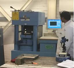
Figure 12 – Compressive strength and tensile splitting test machine

The machine applies a gradual compressive load to the specimen, applying the load too quickly would simulate dynamic loading. The rate of loading in this experiment was 6kN/s in accordance with clause 6.2 of BS EN 12390-3 for a 100mm cube. At peak load i.e., the load just before failure, the test machine will record the load application to allow the compressive strength to be calculated using Equation 4

fc= FAc

Equation 4

Where;

fc  is the compressive strength, in MPa (N/mm²)

F is the maximum load at failure, in N

Ac  is the cross-sectional area of the specimen on which the compressive force acts

For the test to be classed as successful, the test specimen must fail in a particular manner. Tested specimens should show the characteristics shown in Figure 13.

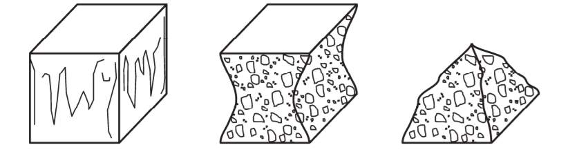
Figure 13 – Failure conditions of compressive strength test

The image to the left of Figure 13 depicts vertical cracking of the concrete surface, the middle image shows the remaining shape after the cracked/loose material is removed and the last image is the shape once the section has been vertically pulled apart. The first two images were true for this experiment, but the last could not be confirmed as the failure specimen was still too strong to separate by hand. The results of the compressive tests are presented in Table 9 and depicted in Figure 14.

Concrete Grade	Cube No	Max Load: F (kN)	Compressive Strength: fc (N/mm2)	Average Compressive strength: fc (N/mm2)
C30	1	448.92	44.892	45.558
	2	462.24	46.224
C70	1	668.68	66.868	58.4185
	2	499.69	49.969

Table 9 – C30 and C70 compressive strength test results

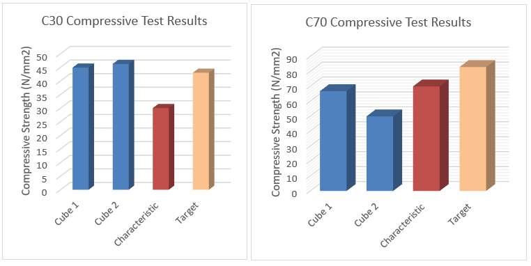
Figure 14 – C30 & C70 Compressive Strength Test Results

4.5.1 Analysis of Results

The 14-day test results show both specimens of the C30 mix has already achieved the required characteristic strength and exceeded the target strength. Neither tests for the C70 specimens achieved the target strength or even the characteristic strength. Cube 1 appears satisfactory as it has almost achieved the required characteristic strength after 14 days, however Cube 2 is approximately 70% of the characteristic strength and only 60% of the target strength.

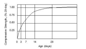
Figure 15 – Typical strength gain curve (Camp, 2017)

Based on a typical strength gain curve of concrete as shown in Figure 15, Cube 2 of the C70 mix should have achieved approximately 85% of its strength. Based on the strength gain curve, it is predicted Cube 2 will only have had a 28-day strength of approximately 60 N/mm², which is below the specified characteristic strength. The mix itself appears to be satisfactory due to the Cube 1 results. This is a practical example as to why you test more than one specimen and design to a higher target strength. The reduction in strength could be due to inadequate compaction of the concrete when it was placed in the mould.

4.6 Tensile Splitting Test

Tensile splitting tests are completed in accordance with BS EN 123960-6. The test is completed by applying a compressive load via a steel plate which has a curved edge at the interface with the concrete specimen.

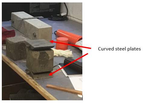
Figure 16 – Tensile Splitting Test

By loading the specimen via a curved plate causes a concentrated loading along a narrow length. The resulting orthogonal tensile force cause the specimen to fail in tension. The load is applied via the same test machine as used in the compressive strength test. As before, the load application should be gradual. A constant stress rate between 0.04 – 0.06 MPa/s should be adopted (BSI, 2009). A rate of 5kN/s was adopted for this test.

The test machine will record the peak load before failure and the tensile splitting strength can be calculated from Equation 5

fct= 2.F(π.L.d)

Equation 5

Where;

fct is the tensile splitting strength (N/mm²)

F is the maximum load (N)

L  is the length of the line of contact of the specimen (mm)

d is the designated cross-sectional dimension (mm)

The test results of both C30 and C70 mix are presented in Table 10.

Concrete Grade	Cube No	L (mm)	d (mm)	Fmax (N)	Tensile Strength: fct (N/mm2)	Average Tensile Strength: fct (N/mm2)
C30	3	100	100	69840	4.446	4.286
	4	100	100	64810	4.126
C70	3	100	100	59880	3.812	4.128
	4	100	100	69790	4.443

Table 10 – C30 & C70 Tensile Strength

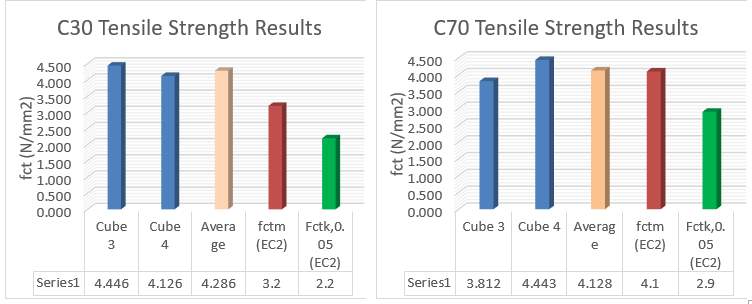
Figure 17 – C30 and C70 Tensile Strength

4.6.1 Analysis of Results

When comparing the average results of both the C30 and C70 mix, both mixes are almost identical. Larger differences can be noted when reviewing Cube 3 of the C70 mix, which is significantly lower than the respective Cube 4 result or even the C30 cube results. However, both average results are greater than the respective mean axial tensile resistance (f_ctm) provided in Table 3.1 of Eurocode 2, with the C70 mix almost identical to the value provided in EC2 (BSI, 2015). In addition, all cubes achieve a higher tensile strength than the characteristic tensile strength, for which less than 5% test specimens are expected to fail, f_ctk,0.05(BSI, 2015). The chosen value of f_ctm and f_ctk,0.05 are based on the average cube compressive strengths from section 4.5 (C30 mix = 45N/mm2; C70 mix =60 N/mm2). It is worth noting that the C30 mix appears to be over performing.

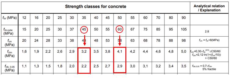
Figure 18 – Table 3.1 from EC2

4.7 Flexural Strength Test

Flexural strength test is completed in accordance with BS EN 12390-5. A 3-point bending test was adopted for this test which incorporates two supports and one point load located in the midspan of the beam. Again, the rate of loading applied to the beam has to be controlled. BS EN 12390-5 specifies a rate of loading between 0.04 – 0.06 Mpa (BSI, 2009) and the test machine records the maximum load (F) at failure.

For a 3-point bending test, Equation 6 is used to calculate the flexural strength

fcf= F.Id1.d22

Equation 6

Where;

fcf is the flexural strength (Mpa)

F is the maximum load (N)

I is the distance between the supporting rollers (mm)

d1/d2 lateral dimensions of the specimen (mm)

The results of the test have been presented in Table 11

Concrete Grade	Beam No	I (mm)	d1/d2 (mm)	F (N)	Flexural Strength: fcf (Mpa)	Average fcf (Mpa)
C30	1	400	100	2325.26	0.930	0.880
	2	400	100	1560.27	0.624
	3	400	100	2711.72	1.085
C70	1	400	100	2410	0.964	0.906
	2	400	100	2258.32	0.903
	3	400	100	2126.08	0.850

Table 11 – C30 and C70 flexure Strength

The average results for both the C30 and C70 mix have been graphed in Figure 19

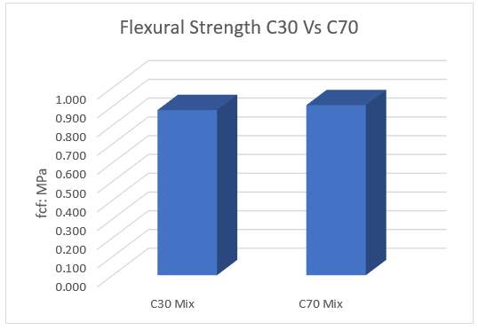
Figure 19 – C30 and C70 flexure strength

4.7.1 Analysis of Results

Both the C30 & C70 mix have similar flexural resistance, with the C70 marginally higher. However, both resistances are extremely small and are <1Mpa. This is surprising considering a bending test will causing the beam to fail in tension, and section 4.6 has already concluded the tensile splitting resistance of both mixes to be approximately 4Mpa.

It is known concrete preforms poorly in tension, the above results further confirm this, but also highlights concrete preform worse in flexure. If a material was homogenous and defect free, the tensile and flexure resistance should be similar. However, concrete is not strictly homogenous, and cracking will propagate at underside of the beam when subject to bending. The cracking is also at the position of the extreme fibres where the tensile force is highest and therefore results in early failure.

4.8 Fracture Energy

Section 4.7 has shown how a test specimen failed before achieving its ‘theoretical capacity’ and that this reduced capacity was due to the propagation of cracks. Griffith was the first person to realise a materials uniaxial tensile resistance cannot solely be used for determining failure resistance and leads into a relatively new field of engineering called fracture mechanics. Fracture mechanics is the field which studies the propagation of cracks i.e. determining whether a pre-existing crack can grow. The energy required to do this is called the fracture energy and is described as the energy required to crack a unit surface area.

There are three main modes of crack propagation 1) opening 2) In-plane shear 3) out of plane shear. The failure mode considered in this investigation will be mode 1 i.e. the opening of a crack.

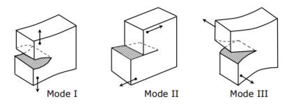
Figure 20 – Crack modes (Dascalu, 2011)

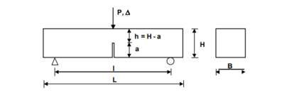
To determine the fracture energy of a specimen, a 3-point bending test is completed on a notched beam. A notch is included to represent an existing crack or defect. Fracture mechanics studies the propagation of cracks and therefore an existing crack/defect has to be simulated. The test specimen is shown in Figure 21.

Figure 21 – Three-point bending test

Where;

L is the length of the beam (500mm)

B is the breadth of the beam (100mm)

H is the depth of the beam (100mm)

a is the depth of the notch (50mm)

h-a is the depth of the ligament (50mm)

l is the effective span (400mm)

The beam has two transducers fixed on either side of the beam to record displacement. A constant rate of deflection is applied to the beam and the corresponding load is recorded by the testing apparatus.

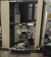
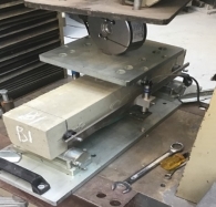
Figure 22 – Three-point bending test machine  Figure 23 – Three-point bending test apparatus

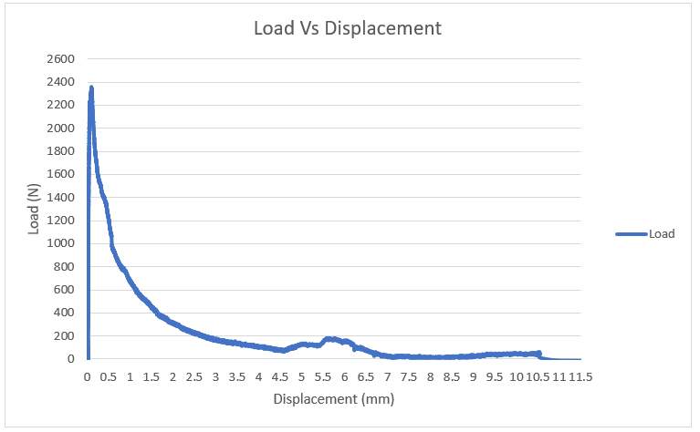
By continually recording displacement and corresponding loading, a load/displacement curve can be plotted. Plotting a load/displacement curve allows the fracture energy to be determined using Equation 7, where the integral relates to the area under the load/displacement curve up until the point of rupture.

           

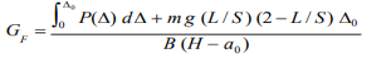
Equation 7

Where;

L, B, H is defined above

P  load (N)

d∆  displacement (m)

m is the mass of the specimen between supports (kg)

S  is the effective span (m)

∆₀ is the displacement at rupture (m)

a₀ notch depth of the beam (m)

Most parameters above are constant between samples. The variables between tests relate to the area under the corresponding load/displacement curve and the maximum displacement at rupture. There is also a minor difference in densities when comparing the C30 and C70 mix. The constant terms are presented in Table 12.

Parameter	Value
Length (L)	0.5m
Breadth (B)	0.1m
Height (H)	0.1m
Effective span (S)	0.4m
Notch depth (ao)	0.05m
Mass (m) – C30 mix	9.357kg
Mass (m) – C70 mix	9.249kg

Table 12 – Fracture energy standard parameters

The calculated fracture for each beam is presented in Table 13.

Concrete Grade	Beam Number	∆0 (m)	∫0∆0P∆d∆ (Nm)	GF   (GPa.m)	Average GF   (GPa.m)
C30	1	0.0106	2.470	675.509	418.4194
	2	0.0030	1.032	258.643
	3	0.0042	1.246	321.107
C70	1	0.0031	1.088	269.678	325.3081
	2	0.0062	1.730	451.862
	3	0.0028	1.038	254.385

Table 13 – C30 and C70 fracture energy results

4.8.1 Analysis of Results

When considering the average results, it can be seen the C30 mix has a larger fracture energy than the C70. However, on review of the results in isolation it is not consistent to say that the C30 mix always required more energy to rupture. In addition, C30 Cube 1 appears to be significantly higher than the rest of the values, and an error in the result could be obscuring the overall conclusion.

If C30 beam 1 is reduced in line with other results, overall there is not a large difference, and one would have expected a clearer divide between the results. This may be due to the compressive strength of the mixes, as noted in section 4.5, the C30 mix seems to be overperforming whereas the C70 mix is slightly under performing therefore the difference is not as large as expected when comparing normal strength concrete (NSC) with high strength concrete (HSC)

However, research does suggest that fracture energy of concrete does marginally increase with compressive strength, although failure is more brittle (K.P. Vishalakshi, 2018). This research was completed on a range of concrete strengths up to a compressive strength of 80 N/mm² and showed an increase in fracture energy with compressive strength. These results are slightly surprising, and one would expect this trend would fail especially when concretes of >100Mpa are considered.

Fracture energy and the propagation of a crack is closely linked with the fracture process zone (FPZ). The fracture process zone is show in Figure 24 and is referred to as the damaged zone ahead of a macrocrack. There are numerous processes ongoing within this area, such as matrix microcracking, debonding of cement-matrix interface, which contribute to the energy of the crack (Gdoutos, 2005). However in high strength concrete with increased brittleness show a reduced (FPZ), which therefore do not initiate the energy mechanisms above and result in reduced fracture energy (Prasad, 2001)

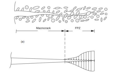
Figure 24 – Fracture Process Zone (Gdoutos, 2005)

This is because in normal strength concrete the weakest part is the interphase between the aggregate and cement matrix, and the crack path goes around the aggregate. Whereas in high strength concrete, the water/cement ratio is reduced, and the strength of the cement matrix is increased, therefore the aggregate can be the limiting strength parameter and the crack can travel through the aggregate resulting in a shorter crack path and a more brittle rupture

Another observation is one would expect the peak load achieved in the C70 mix to be greater than the C30 mix, but when comparing the average peak loads achieved, the C30 mix is marginally higher. This would suggest tensile strength is the limiting strength parameter as both tensile resistances are in section 4.6 are almost identical, but again the C30 mix is marginally higher. Theoretically, the tensile strength of concrete would increase with compressive strength, which would mean a higher peak load should be possible for the C70 mix, however this is offset by increased brittle behaviour which results in small deformation and therefore the difference in area under the load/displacement is marginal.  However to validate this theory would require an increased number of tests to analyse.

5 Brittleness

The measure of brittleness or ductility of a material is the same. It is a measure of the materials ability to undergo plastic deformation prior to rupture. Materials which undergo small deformations are referred to as being brittle, in contrast materials which sustain large deformation are classed as ductile. In design, it is beneficiary for a material to have good ductility. This is because sudden failure is avoided, and as the material undergoes plastic deformation, this provides a visual indicator to occupants, or engineers to highlight potential failure is imminent. A ductile material is also more economical in design, it allows engineers to utilise the plastic capacity of materials, and consider moment redistribution in indeterminate structures, which requires the formation of a plastic hinge to sufficiently rotate and redistribute the load to less stressed areas.

Brittleness is therefore an important material parameter, in this report, the author has considered Bache H.H method of determining the brittleness based on Equation 8 and Peterson P.E (1980) method of determining the characteristic length of the material based on Equation 9.

5.1 Bache Method

As mentioned above, Bache H.H defined the brittleness parameter B in large bodies as the ratio of the characteristic bulk deformation proportional to the characteristic zone deformation and for large bodies and can be calculated based on Equation 8 (Marinelli, 2018).

B=Dft2EGF

Equation 8

Where;

D maximum aggregate size

Ft tensile strength

E dynamic elastic modulus

G_F fracture energy

The brittles of both the C30 and C70 samples have been calculated and the results are presented in Table 14.

Concrete Grade	Beam No	ft	Ed	Gf	B	Average B
C30	1	4.286	42.014	675.509	0.012945559	0.024660833
	2	4.286	42.014	258.643	0.033810464
	3	4.286	42.014	321.189	0.027226477
C70	1	4.128	41.189	269.677	0.030674715	0.027166849
	2	4.128	41.189	451.862	0.018307106
	3	4.128	41.189	254.385	0.032518726

Table 14 – C30 and C70 brittleness index

5.2 Characteristic Length

The characteristic length is also an indicator of a materials ductility or brittleness. It involves three parameters which are specific to the mix, elastic stiffness (E), tensile strength (ft) and fracture energy (Gf).

Research is currently being undertaken to determine new design principles when dealing with high strength concrete which are based on a concretes mix characteristic length as opposed to conventional compressive strength. Current design principles ignore the tensile resistance of concrete, which results in higher minimum areas of reinforcement, which increase with compressive strength. By designing based on the characteristic length allows the actual ductility of the mix to be accounted for (Karihaloo, 2015). This will be useful as mix designs evolve to counter the brittle behaviour of high strength concrete by addition of additivities such as steel fibres.

The characteristic length can be calculated using Equation 9. Higher values of characteristic length relate to increased ductility, whereas lower values relate to increased brittleness

lch= EGfft2

Equation 9

Where;

l_ch is the characteristic length

E  is the elastic modulus

Gf is the fracture energy

Ft is the tensile strength

The static elastic modulus of the samples has been estimated based on standard beam deflection formula as show in Equation 10.

d= 48 E IL3

Equation 10

Where;

P  is the applied load

d  is the recorded displacement at the applied load

E  is the elastic modulus

I  is the second moment of area

L  is the length

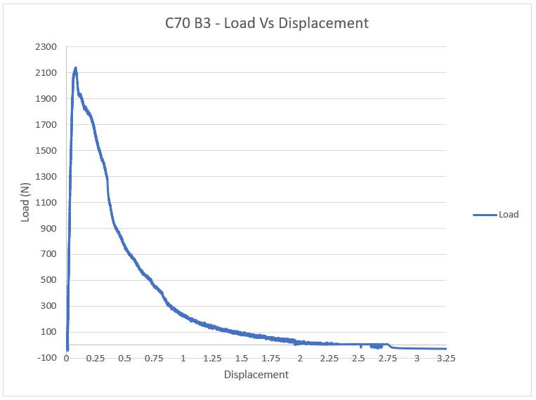
The load/displacement curve was used to determine a suitable range where the elastic modulus could be determined as shown in Figure 25.

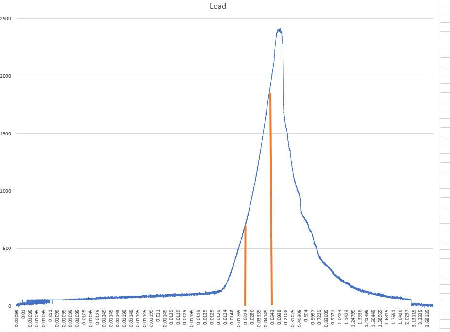
Figure 25 – Typical load/displacement curve

A data entry was selected by reviewing the results within a range and picking a data entry which appears consistent with the graph i.e. a value would only be selected if it appeared to be ascending in the same increments as the results above and below.  The calculated values of E are presented in Table 15. The author notes this is not a robust measurement of E but is suitable for the purpose of highlighting the differences in characteristic length between the C30 and C70 mix.

Concrete Grade	Beam No	L (mm)	I (mm3)	d (mm)	P (N)	E   (N/mm2)	Average E (N/mm2)
C30	1	400	8.33E+06	0.0343	1386	6465.31	6551.64
	2	400	8.33E+06	0.03385	1130	5341.21
	3	400	8.33E+06	0.046195	2266	7848.39
C70	1	400	8.33E+06	0.0586	2160	5897.611	5681.127
	2	400	8.33E+06	0.056886	1795.42	5061.25
	3	400	8.33E+06	0.03695	1405.14	6084.52

Table 15 – C30 and C70 Elastic modulus

Therefore, by using the calculated values of elastic modulus it is possible to determine the characteristic length using Equation 9, the values of which are presented in Table 16.

Concrete Grade	Beam No	ft (N/mm2)	E (N/mm2)	Gf (N/mm)	lch (mm)	Average lch (mm)
C30	1	4.286	6465.306	0.6755	237.743	150.056
	2	4.286	5341.211	0.2586	75.202
	3	4.286	7848.391	0.3212	137.223
C70	1	4.128	5897.611	0.2697	93.356	106.150
	2	4.128	5061.253	0.4519	134.241
	3	4.128	6084.516	0.2544	90.853

Table 16 – C30 and C70 characteristic length

5.3 Analysis of Results

Based on the data presented in Table 14 and Table 16, it is clear the C70 concrete is more brittle than C30, which is what current research suggests, that an increase in compressive strength results in increased brittleness. One reason for this may be due to the water/cement ratio. It has been shown that reducing the water/cement ratio results in a reduction in the fracture energy and therefore an increase in brittleness (Morteza H.A. Beygi, 2013). The C30 mix design had a water/cement ratio of 0.6, whereas the C70 mix was only 0.32. The conclusion that the C70 mixes are more brittle appears to be supported by the lab data graphed in Figure 26. The C70 mixes are depicted by shades of blue whereas the C30 mixes are shades or red. The graph suggest the C70 mix achieved relatively small deformations prior to rupture, demonstrating increased brittle behaviour.

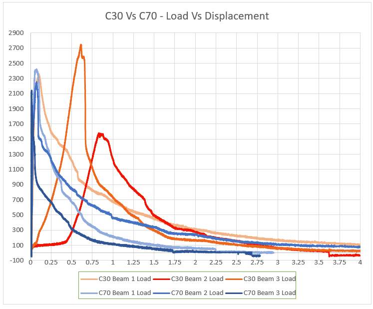
Figure 26 – C30 Vs C70 – Load/Displacement

5.4 Critical Intensity Factor (Fracture Toughness)

Fracture toughness is a measure of a materials resistance to crack propagation (Gdoutos, 2005). A higher fracture toughness value means greater resistance. It is also an indicator of brittleness as one of the parameters is the critical strain energy release rate (Gc). A brittle material will tend to have a reduced energy release area as it will rupture under smaller deformations. Therefore, a lower Fracture Toughness, is an indicator a material is more brittle.

By determining the fracture energy of a specimen, it is possible to determine the fracture toughness KIc , based on Equation 11.

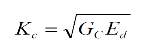           Equation 11

Where;

Gc  is the critical strain energy release rate

Ed is the dynamic modulus

The fracture toughness values have been calculated for the C30 and C70 beam specimens and presented in Table 17

Concrete Grade	Beam No	Ed	Gc	Kc (N/mm3/2)	Average Kc
C30	1	42.0137	675.5086	168.4655	129.6245
	2	42.0137	258.6429	104.2428
	3	42.0137	321.1887	116.1651
C70	1	41.1893	269.6775	105.3936	114.7269
	2	41.1893	451.8617	136.4253
	3	41.1893	254.3851	102.3618

Table 17 – C30 and C70 Fracture toughness

5.4.1 Analysis of Results

Based on the values presented in Table 17, the C30 concrete grade has a slightly higher fracture toughness than the C70 grade. This is to be expected as we have already determined C70 is more brittle than C30 and therefore the critical energy release area is less. This means that the failure state stress for the C30 should be theoretically higher than that of C70 mix when considering Equation 12.

σf= KIc√πa

Equation 12

Where;

σf  is the failure state stress

K_IC is the fracture toughness (mode 1)

√πa is a geometrical parameter of the crack considered

Therefore, when considering an identical crack geometry, the failure state stress increases with K_IC. The above equation is when considering an internal crack, but the principle is the same for a surface crack in that higher fracture toughness increases the failure state stress

6 Conclusion

The fundamental aim of this experiment was to highlight the difference in fracture energy between normal strength concrete (NSC) and high strength concrete (HSC) and introduce the principles of fracture mechanics.  Overall, it has been shown that the energy accommodated by NSC prior to rupture was greater than HSC, but a rogue result may have obscured this result. By neglecting this result, or reducing it in line with the other values, the difference in fracture energy between the mixes is marginal.

With respect to brittleness, it has been established that C70 concrete does appear to be more brittle. The reason for this is believed to relate to the reduction of the water/cement ratio in the C70 mix. The reduced water/cement ratio increases the strength of the cement matrix and means the aggregate is sometimes the limiting strength parameter, resulting in a more direct crack path through the aggregate. However, the author was unable to review the C70 test specimen to confirm, but the theory does coincide with current research.

Fracture toughness has been shown to be larger in the C30 mix in comparison to the C70 mix, but as the main parameter for determining fracture toughness is fracture energy, it is susceptible to the same rogue result as described above. Again the values would be similar, however the author would have envisaged a reduction in fracture toughness with increased compressive strength. These results may be due to the fact the average peak load achieved in C70 mix is approximately the same as the C30, with the C30 mix marginally higher. This would suggest the peak load is limited by  the concrete tensile resistance, as detailed in section 4.6, the tensile strength of both mixes were almost identical, with the C30 mix being marginally higher. If the peak load is limited by tensile strength, and both mixes have the same resistance, it may explain why there is little difference.

Overall the differences in comparing the two concrete mixes appear to be marginal, but the brittleness of concrete will increase with higher strengths mixes. Modern developments in concrete technology have allowed the production of concrete with ultra-high compressive strengths in excess of 100MPa. Concrete with such a high compressive strength present extremely brittle behaviour (Gdoutos, 2005) and the application of fracture mechanics is required to understand crack propagation and therefore fracture toughness to control crack growth via new design mixes or design principles to allow engineers to avoid brittle failures.

7 Bibliography

BSI, 2000. BS EN 12350-2:2009. Testing fresh concrete. Slump-test.

BSI, 2009. BS EN 12390 Testing hardened Concrete Part 6: Tensile splitting strength of test specimens, s.l.: BSI.

BSI, 2009. Testing Hardened Concrete. Part 2: Making and curing specimens for strength tests.

BSI, 2009. Testing Hardened Concrete: Part 5 – Flexural strength of test specimen, s.l.: BSI.

BSI, 2015. Eurocode 2: Design of Concrete Structures Part 1-1: General rules and rules for buildings, s.l.: BSI.

Building Establishment Research, 1997. Design of normal concrete mixes. 2nd ed. s.l.:Construction Research Communications Ltd.

Camp, C., 2017. CIVL 1101 – Properties of Concrete. [Online]
Available at: http://www.ce.memphis.edu/1101/notes/concrete/section_3_properties.html

Dascalu, C., 2011. An introduction to fracture mechanics.

Gdoutos, E., 2005. Fracture Mechanics: An Introduction. s.l.:Springer.

John T. Petro Jr., J. K., 2011. Construction and Building Materials. Detection of delamination in concrete using ultrasonic pulse velocity test, 26(1), pp. 574-575.

K.P. Vishalakshi, V. R. S. S. R., 2018. Engineering Fracture Mechanics. Effect of type of coarse aggregate on the strength properties and fracture energy of normal and high strength concrete, pp. 52-60.

Karihaloo, B. L., 2015. A new approach to the design of RC structures based on characteristic length.

Marinelli, A., 2018. SECTION 2 – FRACTURE PROPERTIES OF CONCRETE. MSc ADVANCED STRUCTURAL ENGINEERING – CTR11118 Advanced Structural Concrete.

Morteza H.A. Beygi, M. T. K. I. M. N. J. V. A., 2013. Materials and Design. The effect of water to cement ratio on fracture parameters and brittleness of self-compacting concrete.

Online Civil Engineering, 2010. Slump Test. [Online]
Available at: http://civil-online2010.blogspot.com/2010/02/slump-test.html
[Accessed 2018].

Prasad, G. R. &. B., 2001. Fracture Mechanics of Concrete Structures. Fracture process zone in high strength concrete.

Xiaobin Lu, Q. S. W. F. J. T., 2013. Construction and Building Materials. Evaluation of dynamic modulus of elasticity of concrete using impact-echo method, Volume 47, p. 231.

Appendices

Appendix A – C30 & C70 mix designs

C30 Mix Design

C70 Mix Design

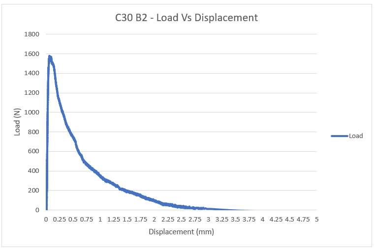
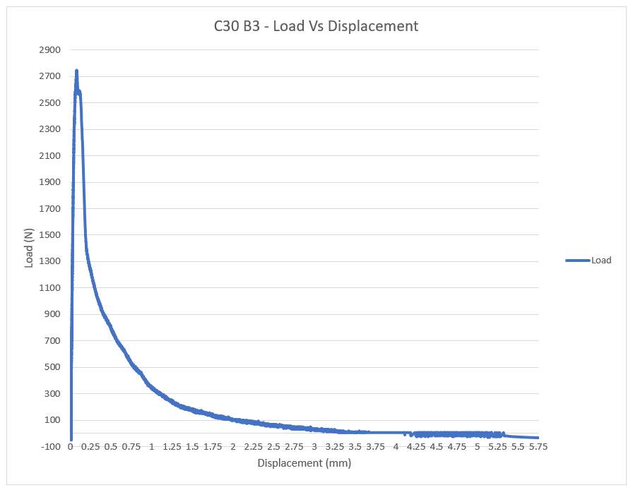
Appendix B – C30 Load/Displacement Graphs

C30 Beam 1

C30 Beam 2

C30 Beam 3

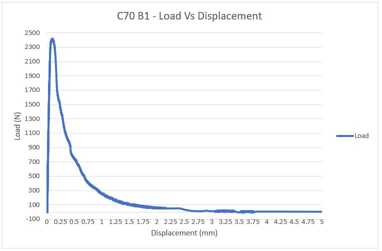
C70 Beam 1

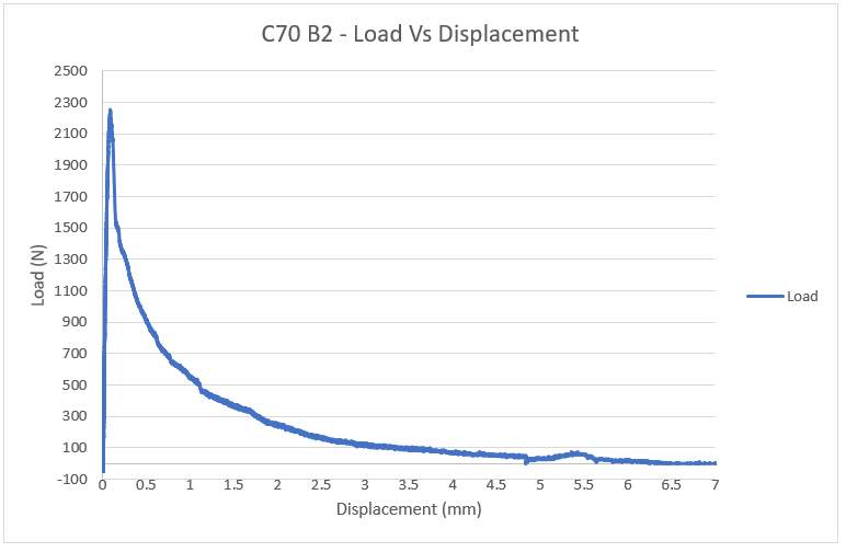
C70 Beam 2

C70 Beam 3