Impact of Localised Energy Systems on Low Voltage Distribution Systems
Info: 6320 words (25 pages) Dissertation
Published: 16th Dec 2019
Tagged: Energy
Chapter 1
Integration of local energy in the distribution network could provide economic benefits to people or organisations in a specific geographical area or community and assist in securing electricity supply[1]. Local energy systems is developed to target local needs and takes advantage of the unique opportunities available in each area.
The introduction of local generators will encourage an increase of renewable energy sources (photovoltaic, hydro and wind power). These renewable sources offers the benefits of power security and carbon emission reduction [2]
However, with significant penetration of local generations, the power flow in the distribution network may be become reversed[3]. This depend on the relative magnitudes of the real and reactive network loads compared to the generator outputs and any losses in the network. This change in grid behaviour create a new challenges for the utility in determining how to plan, design, and operate distribution systems that were not designed for the application of local generation. Some of the technical challenges posed to electric utilities were analysed and discussed in this thesis namely network voltage changes, network losses and transformers loadings.
This thesis investigated the impact of localised energy systems on LV electricity distribution systems. Distributed generators were integrated in three different localised energy systems. The steady state voltage profile, network losses and transformers loading were determined and compared in the three networks. Lastly, the total capacity (units) of DG that could be installed by individual customers was investigated.
The local distribution network area considered in this chapter is a LV part of the UK generic distribution network model described in [4] with installed local generators.
1.1.1 NETWORK VOLTAGE CHANGES
Introduction of distributed generation (DG) may cause variation in the network voltage. This may influence power quality in the network. It is the obligation of the distribution network operator (DNO) to supply its customers at a voltage within specified limits. This specified voltage values vary from country to country. In the UK the electricity supply limit is +10% -6% at 230V[5].
The difference between the lower voltage limit and the upper voltage limit is the available voltage band within which the node voltages may vary in a network. This requirement often determines the design of the distribution circuits.
For a lightly loaded distribution network the approximate voltage rise (∆V) due to the generator is given by[5],[3].
∆V=PR+XQV (1)
Where: V = nominal voltage of the circuit
, P = active power output of the generator, Q = reactive power output of the generator, R = resistance of the circuit, X = inductive reactance of the circuit. In the network shown in Fig3.1, the power flow may not be unidirectional. According to the size and production of the DG unit, and network load demand, power flow in the network may be bidirectional.
With bidirectional power flow, challenges such as a voltage rise may occur. Voltage rise due to the connection of DG in the distribution networks can be an obstacle for connecting DG, especially in the rural areas with long overhead lines.
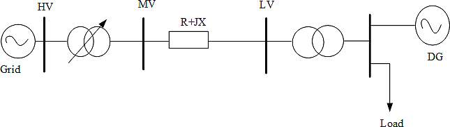
Fig 3.1: Radial distribution network with a DG unit [6]
1.1.2 NETWORK LOSSES
Electricity transported to distribution network is lost within the network components. The estimate of electrical losses on distribution network is calculated as the difference between power entering and exiting the network. Power lost across the distribution system is considered as electrical loss. There are number of factors that affect power losses in the distribution networks such as (i) parameters of transmission lines i.e. length, type, size, material of cables etc. (ii) number and characteristics of electrical device i.e. transformers, conductor etc. (iii) types of connected loads in the systems[7]. Losses on the power system depend upon the current flow in the line and also line parameters. The real power loss is I2R and reactive power loss is I2X. All system losses are unavoidable but they can be minimised by planning and operating distribution networks in optimal way.
The Distribution losses are important from the Distribution Network Operator (DNO) point of view since power losses are an economic concern and have to be minimized[8]. There are many methods of loss reduction techniques used like feeder reconfiguration, capacitor placement, high voltage distribution system, conductor grading, and DG placement
Distribution loss mainly depends upon the network configuration and loads connected[10]. The increase in the DG penetration leads to a significant reduction power losses. The simulation provide the save penetration level for distribution losses reduction. The maximum losses reduction level suggests the DNO companies to make improvement in planning and additional investment in distribution system infrastructure to minimize losses.
1.1.3 TRANSFORMER LOADING
Transformers are generally rated in kVA or MVA. They have long thermal constants and thus can be overloaded for short periods of time without causing overheating or significant damage.
Transformers are generally chosen to match the expected maximum demand and are not normally operated at a significant proportion of their thermal limit, partly because standing (no load) losses are significant and so the efficiency of a lightly loaded transformer is poor. Thus, in areas with very high penetrations of embedded generation, thermal limits of transformers can resist further installation.
Most transformers can accommodate reverse power flow, up to the normal forward rating, without a problem. However, there are some (not many) on-load-tap changers that have very limited reverse-power capability. Furthermore, some automatic voltage regulators associated with on-load tap-changers can be affected by reverse power flow.
Thus, the thermal limits of existing transformers are not normally a limiting factor in the installation of distributed generators, unless the installed capacity of generators exceeds the maximum demand in the area served.
The increase in the residential or commercial loads and penetration of DG will impact the load current flowing in the distribution system. The transformer loading beyond the rated capacity due to increase load current will affect the insulation withstand capacity of and may result in insulation breakdown followed by flashover. This is a critical condition and needs to be examined before wide scale adoption of both DG.
1.2 the uk generic distribution network
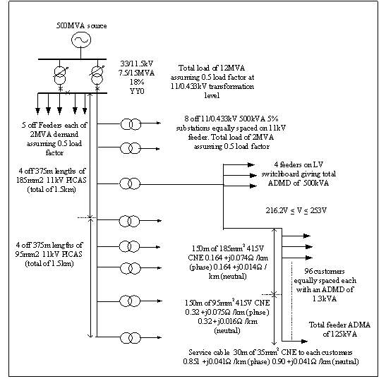
The UK generic network (UKGDN) model, representative of UK distribution networks is used for this study. This distribution network model is used by many distribution network operators. It consist of a 500 MVA three phase 33kV ideal voltage source, connected to two 33/11.5kV 15MVA YY0 transformers, and eight 11kV outgoing feeders substation. Each feeder supplies 11/0.433kV transformer which ultimately fed the local energy systems as shown in Fig 3.1
The network was modelled in NEPLAN software environment defining all the parameters as provided in [4]. NEPLAN is a versatile power system analysis tool that is able to perform load flow analysis for multiple bus networks.
1.2.1 LOCALISED ENERGY SYSTEMS
Three different local energy systems are defined in this system namely, LES1 with residential load, LES2 with commercial load, while LES3 has mixed load (a combination of residential and commercial loads). These are represented in the network as shown in Fig3.1.
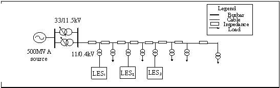 Fig 3.1. Distribution system with Localised energy systems
The next section will consider each of the local energy system and compare their impact on the electricity distribution system at different level of DG and EV penetrations.
1.2.1 LOCAL ENERGY SYSTEMS1 (LES1)
The residential network model is taken from [11], which is also based on the 2003 report by PB power [4] for the department of trade and Industry. Each 11KV feeder in the network is allocated 2MVA at peak load. One 400V feeder is replaced with a residential distribution network supplying 384 homes with a single-phase electrical supply at 230V +10%/-6%, 50Hz.
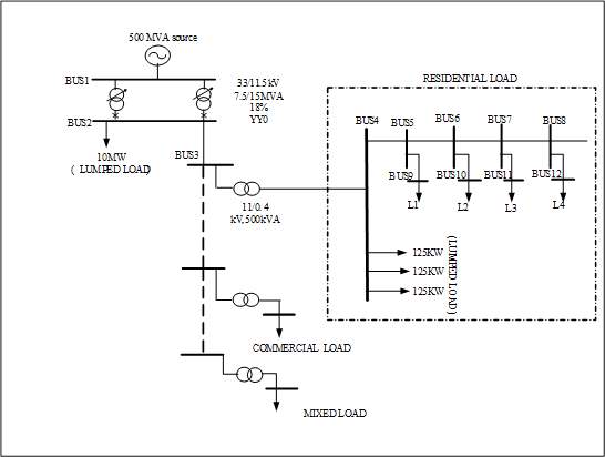
Fig 3.2: Generic UK Network with LES1[4]
This load is assumed to be uniformly distributed among each customer.
One of this LV feeders is modelled in detail as shown in the Fig.3.2. The other three feeders groups are replicated. Considering three lumped values, each lump encompasses the cumulative load of 96 individual consumers.1.2.2
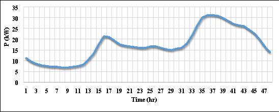
Fig3.3: A typical residential half-hourly load profile[12]
Source: Electricity Association, (provided to UKERC Courtesy of Elexon Ltd)
1.2.2 LOCAL ENERGY SYSTEMS 2 (LES2)
As shown in Fig.1, one 400V feeder was replaced with a commercial feeder of sixteen (1) offices with a maximum and minimum loading of 19.275KVA and 7.5kVA. The 16 offices within the model are distributed evenly between four segments. The load profile has been provided by Electricity Association to UKERC Courtesy of Elexon Ltd, to enable the modelling of office buildings within this study (as shown in Fig.3.4). Due to the types of equipment they contain, offices present a partially capacitive load to the network. The average office has a power factor of approximately 0.85.

Fig 3.4: Generic UK Network with LES2
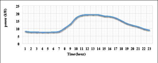
Fig. 3.5: Commercial load profile [12]
Source: Electricity Association, (provided to UKERC Courtesy of Elexon Ltd)
1.2.3 Localised energy system 3 (LES3)
The low voltage network consisted of a housing estate with 63 residential properties and one commercial property and is based on a real Cardiff network .This is an urban area so the network was connected by underground cable; CU-copper underground and WC-Wavecon are used. The Network is shown in Fig.3.6
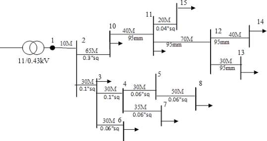
Fig. 3.6: Circuit diagram of Localised Energy System 3 (LES3)
The above figure shows the network consists of 15 nodes and a distribution transformer (500 kVA) with a demand of 127 kVA. The commercial load in the network is represented by node 15. The network data is given in Table1. (Appendix)
A total of 64 consumers are listed on this housing estate, 63 are residential with 1 listed as a commercial building. Each residential consumer is denoted as a type 1 consumer by WPD. This specific type is known as unrestricted domestic and has an annual consumption of 4000kWh. Also included in the network, along with residential properties, is one commercial building. This commercial building is denoted as a type 7 non-domestic with a load factor between 30-40% and an annual consumption of 50000 kWh.
1.3. CASE STUDIES
In order to investigate the impact of DG on LV electricity distribution system, the following procedure must be followed.
- Analyse the modelled test system without DG connected in the network
- Define the penetration levels (PL): In this case studies, three levels of penetration with respect to the total power of the system are selected (0%, 100% and 200% etc.)
- Connect the Distribution generators (DG) at the optimal location and change the DG penetration level
- Analyse the system again with DG connected in the network.
- Observed the impact on of DG on Voltage profile, Losses and Transformer loading
- Compare the simulation results with and without DG installation in the three Localised energy systems.
Four case studies were defined to analyse the impacts of DG on the distribution systems with localised energy systems:
- Case 1 investigated the impact of DG penetration on network voltage profile.
- Case 2 investigated the impact of DG penetration on network losses
- Case 3 investigated the impact of DG penetration on Transformer loading.
- Case 4 determined the maximum capacity (units) of DG that could be connected by individual customers in the distribution system without violating the DNO permissible voltage limits.
1.3.1 Case-1
Voltage Changes
The first case study investigated voltage changes in the modelled Distribution system as DG are connected. Since load configurations varies in each of the localised energy systems, it implies that the impact of DG on the power systems will varies.
Two different simulations were performed. The first simulation was conducted with zero DG penetration. That is, the power flow analysis was performed with existing grid and the connected loads (normal network operation). The second simulation was performed with 100% DG penetration i.e. all customers have DG installed in their premises. The simulation was repeated for the three localised energy systems.
In accordance with Electrical Safety, Quality and Continuity Regulation 2002, the statutory voltage limits are currently +10%/-6% based on 230V[13]. The simulation results are shown in Fig 3.1, Fig 3.2 and Fig 3.3.
1.3.1.1 DG Related Assumptions Used in the Case Studies
A basic unit of PV are considered to be 1.1 kW for residential customers. Thus for 100% penetration each of the 24X4 residential load is connected with 1.1 kW of PV panels based on the selected DER. The commercial customer each have 5.5kW of PV connected per customers. Uniform penetration among the four segments was considered for both residential and commercial customers (i.e. same penetration per 24 customers and 4 offices).
Simulation Results
LES1: Power flow study was undertaken with a normalized half-hourly load shown in Fig3.3. The time–series load was applied at load position bus 12 (L4) of Fig 3.2. The network components and the details of the connecting cables used in the modelling are shown in Appendix A.
The voltage profile at zero DG reflects the normal working voltage of the system. As shown in Fig 3.1,  the minimum voltage of 0.4355917 kV (1.06 Pu) occurred between 17.30hr and 18.00 hr when customer have arrived from their offices. The maximum voltage of 0.43882 kV happened during 3.30 hour and 4.00 hour when customers are still in their offices. The minimum and maximum allowable voltage limit for low voltage levels being 0.4042 kV (0.94 pu) and 0.473 kV (1.10 pu) respectively.
Since the network is built to keep the voltage below the upper limit at minimum load, the case should not be a problem.
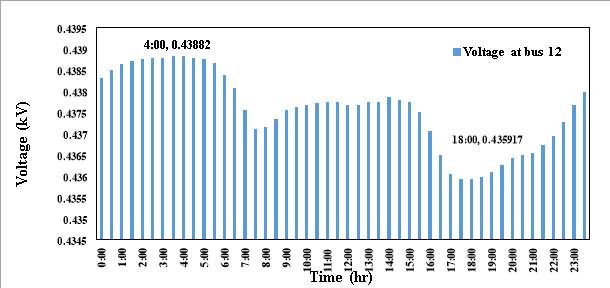
Fig 3.7: Voltage at observation node without DG
In the second simulation, 1.1kW DG units were connected to each of the residential customers representing 100% DG penetration. As shown in Fig.3.9, there was significant increase in voltage when DG was connected. The minimum voltage increased to 0.446045 kV (1.06 Pu) between 17.30hr and 18.00 hr and the maximum voltage increased to 0.448767 kV during 3.30 hour and 4.00 hour.
This is due to DG power cancelling out some or all of the residential load, and some due to excess generator real power flowing back through a mainly resistive network to the distribution transformer
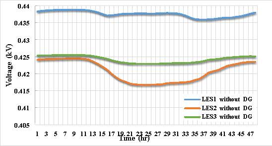
Fig 3.8: Network Voltage at observation nodes without DG
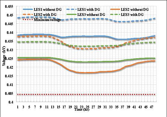
Fig 3.9: Network Voltage at observation nodes with and without DG.
LES2: The network consist of only commercial customers. Due to the type of equipment they contain, offices present a partially capacitive load to the network.The average office power factor is approximately 0.85 (Pabla Book).
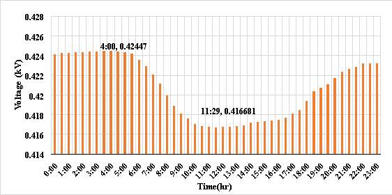
Fig 3.10: Voltage at observation node without DG
The voltage profile at zero DG is shown in Fig.3.2. The minimum voltage at the point of observation is 0.41668 kV (0.969 Pu). This occurred at 11.30am when customer’s load is peak. Also, the maximum voltage of 0.42477 kV (0.987pu) was observed at 4.00am when customers were out of office.
When 5.5kW DG units were connected to each of the commercial customers representing 100% DG penetration. The minimum voltage in the network rose to 0.430439 kV which is an increase of 13.7V while the maximum voltage rose to 0.434 kV representing an increase of 13.01V.
LES3: A combination of residential load and commercial load is connected to the network, in this thesis, was referred to as mixed load. The voltage values without and with DG is represented in Fig 3.3 by solid green line and dotted green line respectively. The maximum voltage rose from 0.429479 kV to 0.434523kV, that is, voltage rose by 5.04V. The minimum voltage rose from 0.426916kV to 0.432416 kV representing an increase of 5.55V.
Case- 2
Network Losses
Power losses in electric power grids are caused by active and reactive power flows through line resistance; the magnitude of the losses depends on the amount of current flow and the line resistance. In this section, power losses have been estimated for an electricity distribution system and compared for three different localised energy systems. The desire of every utilities is to minimise power losses while complying with network voltage limit. Losses are calculated with power flows using three sets of simulation were performed to determine the network losses. The first simulation was conducted with zero DG penetration and the corresponding losses is shown in Fig3.11. Also, the second simulation had 100% DG penetration in the network.
LES1: Over the simulation time, without DG connected in the network, the active power losses are summarized to 0.8849 MWh. When 100% DG penetration was added to the network the losses reduced to 0.7302 MWh. The total loss reduction is 0.1547MWh as shown in Fig. 3.11 and Table, which correspond to 17.48% loss reduction.
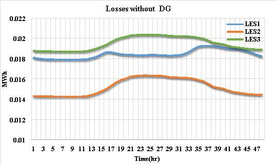
Fig.3.11: Losses without DG penetration.
LES2: The total network losses without DG connected is 0.729MWh. As shown in Table 3.1, the value reduced to 0.6153MWh with 100% DG added to the network. The total loss reduction is 0.1139MWh (15.61%).
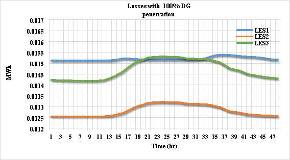 Fig.3.12:
LES3: From Fig 3.12, it was shown that without DG the losses in the network was 0.9351 MWh. The losses reduced to 0.7062 MWh with DG connected to the Distribution network. The green plot shows the variation of the network losses at the point of observation over the 24 hours.
Table 3.1: Losses with and without Distributed generation.
| Type | Losses (MWh) | |||
| 0% DG penetration | 100% DG penetration | Loss reduction | Loss reduction
(%) |
|
| LES1 | 0.8849 | 0.7302 | 0.1547 | 17.48 |
| LES2 | 0.7292 | 0.6153 | 0.1139 | 15.61 |
| LES3 | 0.9351 | 0.7062 | 0.2289 | 24.47 |
Case- 3
Transformer Loading
Distribution transformers connected in the distribution network have specific loading or utilisation capacity and for smooth power supply to customers, it is essential to operate each distribution transformers within safe operating limits designated by DNO.
Therefore, this section investigated the impact of DG penetration on LV distribution transformers that fed the localised energy systems. A power flow calculation for each of the 24 hours of the day is done in the evaluation of transformer loading. The same simulation which has been used for other case study. The maximum power in MVA or the maximum current in Amp (A) must be known for the calculation of transformer loading. For this simulation the rating of the transformer is 500kVA. The first simulation used the grid and the connected load and the second simulation used the grid, connected load and 100% DG penetration. The simulation results are discussed next.
LES1: The simulation results is depicted in Fig.3.13. The blue plot indicate the loading on Transformer T1 of LES1 without DG in the network. From the plot it shown that the transformer varies with time and increases as customers demand is increased. The loading is minimum (85.82%) during the night (between 2am and 4am) and the peak (90.42%) is during the evening time (between 5pm and 6pm).
With DG connected to the network, the transformer’s minimum loading of 66.5% occurred between 3.30am and 4am when most of the residential customers are still sleeping.
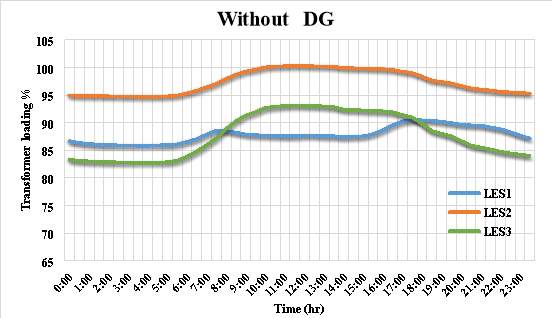
Fig3.13: Network Transformer loading without Distributed generator
At this time only few customers gadget are connected in the network. However, the maximum loading of the transformer (70.9%) occurred between 17.30pm and 18.00pm when the customers demand is at the peak. There is an approximately 20% reduction in loading.
LES2: As shown in Fig 3.13 without DG, the transformer loading varied between 82.66% and 93.12. With DG installed the loading varies between 94.7% and 100.3% for the 24 hours simulation time. From the plot in Fig 3.14, it shown that the minimum transformer loading for the commercial customers (with DG installed) is 64.7% which occurred at 3.00am and the peak (69.6%) occurred at 11.30am.
LES3: From Fig 3.13, it was shown that without DG the maximum loading of the distribution transformer 93.12% 70.51% at 11.30am while the load demand is maximum. Transformer loading was reduced to70.51% at11.30am and 58.02%at 4.00am with DG connected to the Distribution network.
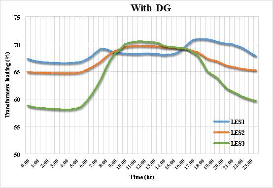
Fig3. Fig3.14: Network Transformer loading without Distributed generator
Case-4
DG Capacity Installed
In this case study the total capacity of DG that could be installed in each localised energy systems was determined. Load flow study was performed to determine network voltage. DGs were installed in the network in increasing penetration order. (50%, 100%, 200% and 300%). In the all the simulations and analysis the statutory voltage limit of +10%and -6% was strictly maintained. Thermal limit of the DT was not exceeded and likewise losses on the line was monitored. The results is presented in Table 3.2
LES1: As shown in Table 3.2., each customer can accommodate 3 units of DG (3×1.1=3.3kW) which represent 300% DG penetration.
LES2: Each of the commercial customers can accommodate or have installed 3 units of DG (3×5.5=16.5 kW), this represent 300% DG penetration as shown in Table 3.2.
LES3: each of the residential customer have installed 4.4 kW of DG (1.1x 4=4.4kW) and each of the commercial customer have installed 4 units of DG (5.5 x4=22kW) as shown in Table 3.2. This represent 400% DG penetration in the network.
Table 3.2: Maximum DG unit per customers
| Network | Voltage increase | Losses Reduction | Transformer loading reduction | DG Unit per customers |
| LES 1 | 10.12 V (2.32%) | 17.48% | 21.5% | 3.3 kW (300%) |
| LES2 | 13.7V (3.28%) | 15.61% | 38.5% | 16.5 kW (300%) |
| LES3 | 5.04V (1.17%) | 24.47% | 39.2% | 4.4 kW (400%) /
22kW (400%) |
Conclusion
In order to
1.2.3.2 DG Related Assumptions Used in the Case Study
Average half-hourly weekdays load profiles were drawn from [Rilwan], with typical minimum and maximum values as 6.78kW and 30.86kW respectively. A basic unit of PV are considered to be 1.1 kW for residential. Thus for 100% penetration each of the 24X4 residential load is connected with 1.1 kW of PV panels based on the selected DER. Uniform penetration among the four segments was considered for residential customers (i.e. same penetration per 24).
1.2.3.1 Assumptions Used in the Calculation Process
There were certain assumptions made during the development of this network
- The domestic loads modelled on the LV distribution network (0.4 kV) are assumed to be uniformly distributed between each customer. For this simulation the extreme cases are investigated. In reality the loads are unlikely to be consistent and a demand factor is applied to estimate average demand.
- The loads are assumed to be purely resistive with unity power factor.
- The switching is assumed to be smooth and the analysis is carried out in the steady state during its operation.
- Generally in a distribution network the loads and DGs are single phase. It is assumed that the load is uniformly distributed among each phase through the network enabling balanced 3 phase operation.
- All the DG sources considered are assumed to be free from harmonics and other distortions.
The assumptions made are significant challenges and are potentially independent research topics. These however are not in the scope of this thesis
1.2.3.2 EV Related Assumptions Used in the Case Study
A basic unit of EV are considered to be 6.6 kW for residential load [15]. Thus for 100% penetration each of the 24X4 residential load is connected with 3.3 kW of EV charger and for the commercial customer each have 6.6kW of EV charger connected per customers. Uniform penetration among the four segments was considered for both residential and commercial customers (i.e. same penetration per 24 customers and 4 offices).
1.3 Methodology
For the study of the network model in Fig 3.1, power flow study is required. The power flow study was carried out in Neplan software. The objective of the power flow study is to performed steady state analysis during normal operation. The main information obtained from this study comprises the magnitudes and phase angles of load bus voltages, real and reactive power flow on the transmission lines, network losses, transformer loadings and power injection at all the buses.
The simulation was carried out to deter aim is to determine the impact on the steady state voltage profile, network losses and transformers loading when DGs are connected to the distribution network. Also the impact of Electric Vehicles (EVs) charging were also study during minimum and maximum loading of the network.
The simulation was done considering the extreme conditions: DG connection at minimum load and EVs charging at maximum load with different levels of penetration. The case studies were conducted under normal operating conditions. There was uniform distribution of generation and EVs charging. With the addition of each the DG source, the voltage of the LV system is expected to rise.
Based on the capacity of the DG the voltage could rise above the nominal value. Using the simulation, the system voltage is monitored with different levels of DG penetration. Normally in a radial network, a voltage drop is expected downstream, due to unidirectional power flow. However, with an addition of a DG at the point of consumption, the required power for each load is generated at the point of requirement resulting in a voltage rise at the point of connection. The UK Electrical Safety, Quality and Continuity Regulations and the national electrical code, specifies the acceptable limits of voltage to be +10% and -6% of the nominal voltage in an LV Network. [17]. This limit helps establish the maximum DG that can be connected to the selected distributed network such that the statutory voltage regulation is maintained. To analyse the network different scenarios are developed. The above discussed parameters are investigated for each network scenario.
Three case studies were defined. Case study 1 represent the first local energy system (LES1), case study 2 represent the second local energy system (LES2), and the Case study 3 represent the third local energy system (LES3. The main characteristics of the case studies are shown in Table
LES1FigureIn the first case study the Fig. 3.11 and Fig. 3.12 show the EV battery aggregated demand profiles per 24 customers when the EVs followed the optimal charging schedules and when the EV battery charging was not managed. The grey bars show the difference between the energy generated by the micro-generators and the residential demand without considering the EV battery demand (values are positive when the generation is higher than the demand). The red bars show the EV battery aggregated energy demand. The black bars show the difference between energy generated by the micro-generators and the total demand (residential demand plus EV demand).
References
[1] Ofgem, “Ofgem’s Future Insights Series Local Energy in a Transforming Energy System Ofgem’s Future Insights Series Local Energy in a Transforming Energy System What is local energy?”
[2] Y. S. Edenhofer, OttmarRamón Pichs-Madruga, “Renewable Energy Sources and Climate change.”
[3] M. A. Mahmud, M. J. Hossain, and H. R. Pota, “Analysis of Voltage Rise Effect on Distribution Network with Distributed Generation,” 2011.
[4] S. Ingram, S. Probert, and K. Jackson, “The impact of small scale embedded generation on the operating parameters of distribution networks,” Dep. Trade Ind., 2003.
[5] N. Jenkins, J. B. Ekanayake, and G. Strbac, Distributed Generation. 2010.
[6] A. Hagehaugen, “Voltage Control in Distribution Network with Local Generation,” no. June, 2014.
[7] M. A. Kashem, A. D. T. Le, M. Negnevitsky, and G. Ledwich, “Distributed generation for minimization of power losses in distribution systems,” 2006 IEEE Power Eng. Soc. Gen. Meet., p. 8 pp., 2006.
[8] Sohn Associates Limited, “Electricity Distribution Systems Losses: Non-Technical Overview,” Rep. Prep. OFGEM, 2006.
[9] M. C. Anumaka, “Analysis of Technical Losses in Electrical Power System ( Nigerian 330Kv Network As a Case Study ),” Int. J. Res. Rev. Appl. Sci., vol. 12, no. August, pp. 320–327, 2012.
[10] Top Energy, “Network Loss Factor Methodology,” 2008.
[11] P. Papadopoulos, S. Skarvelis-Kazakos, I. Grau, L. M. Cipcigan, and N. Jenkins, “Electric vehicles’ impact on British distribution networks,” IET Electr. Syst. Transp., vol. 2, no. 3, p. 91, 2012.
[12] UKERC, “UKERC Energy Data Centre.” [Online]. Available: http://ukerc.rl.ac.uk/DC/cgi-bin/edc_search.pl?GoButton=Detail&WantComp=42&WantResult=&WantText=EDC0000041. [Accessed: 12-Feb-2018].
[13] Department of Trade and Industry, “Guidance on The Electricity Safety, Quality and Continuity Regulations 2002,” Rep. Number URN 02/1544, no. October, pp. 1–47, 2002.
Appendix A
Appendix
Table1. Low Voltage Network Data
| Operating Resistance | |||||||
| Ratings | Phase | Neutral | Phase | ||||
| Nodes | Length(M) | Types | Size | (AMPS) | Ω/1000M | Ω/1000M | Ω/M |
| 5 and 8 | 50 | CU | 0.06”sq | 197 | 0.4637 | 0.4637 | 0.023185 |
| 4 and 7 | 35 | CU | 0.06”sq | 197 | 0.4637 | 0.4637 | 0.0162295 |
| 3 and 6 | 30 | CU | 0.06”sq | 197 | 0.4637 | 0.4637 | 0.013911 |
| 4 and 5 | 30 | CU | 0.06”sq | 197 | 0.4637 | 0.4637 | 0.013911 |
| 3 and 4 | 30 | CU | 0.1”sq | 270 | 0.2758 | 0.2758 | 0.008274 |
| 2 and 3 | 30 | CU | 0.1”sq | 270 | 0.2758 | 0.2758 | 0.008274 |
| 1 and 2 | 10 | CU | 0.36”sq | 514 | 0.0928 | 0.0928 | 0.000928 |
| 1 and SUB | 10 | CU | 0.3”sq | 514 | 0.0928 | 0.0928 | 0.000928 |
| 12 and 13 | 30 | WC | 95mm | 251 | 0.32 | 0.32 | 0.0096 |
| 11 and 12 | 70 | WC | 95mm | 251 | 0.32 | 0.32 | 0.0224 |
| 12 and 14 | 40 | WC | 95mm | 251 | 0.32 | 0.32 | 0.0128 |
| 10 and 11 | 40 | WC | 95mm | 251 | 0.32 | 0.32 | 0.0128 |
| 2 and 10 | 65 | CU | 0.3”sq | 514 | 0.0928 | 0.0928 | 0.006032 |
| 11 and 15 | 20 | CU | 0.04”sq | 156 | 0.7027 | 0.7027 | 0.014054 |
1.1.4 CABLE LOADING
The increase in the penetration of both DG and EV results in larger load which causes increased power flows in the distribution system. Increased power flows consequence for larger amount of current to handle by the distribution cable. The distribution cable will be extremely loaded for extremely loaded for extreme operating conditions of maximum residential load and maximum EV penetration.
The rated continuous current capacity of cable determines the maximum allowable load currents at a referenced ambient temperature, allowable temperature rise and geometry and its installation. During the service operation, cables suffer electrical losses in the form of heat in conductor, insulation and metallic components. The heating due to the line losses sets a thermal limit. If too much current is drawn, conductors may sag too close to the ground, or conductors and equipment may be damaged by overheating. The important parameters for standard operating conditions are temperature. If a bare overhead conductor is loaded continuously above rated ampacity the mechanical strength of the conductor is reduced. This will lead to a loss of mechanical life, not instantaneous failure. If an underground cable is loaded continuously above rated ampacity then the cable insulation will deteriorate causing insulation break down and flashover.
. The Cable resistance is greater than the cable reactance. It is important to note that these change in voltage could cause the Low voltage (LV) systems distribution network to exceed the permissible limits.
Cite This Work
To export a reference to this article please select a referencing stye below:
Related Services
View all


Related Content
All TagsContent relating to: "Energy"
Energy regards the power derived from a fuel source such as electricity or gas that can do work such as provide light or heat. Energy sources can be non-renewable such as fossil fuels or nuclear, or renewable such as solar, wind, hydro or geothermal. Renewable energies are also known as green energy with reference to the environmental benefits they provide.
Related Articles
DMCA / Removal Request
If you are the original writer of this dissertation and no longer wish to have your work published on the UKDiss.com website then please: