Influence of Trim Optimization on Ship Performance and Fuel Consumption
Info: 8259 words (33 pages) Dissertation
Published: 9th Dec 2019
Tagged: EngineeringEnergyMaritime
ABSTRACT
In recent years, because of increasing fuel costs and environmental issues, technology has been working intensively based on achieving vessel optimum trim to increase power saving and reduce greenhouse gas emissions. In this work a simplified ship model was replicated in Ansys Fluent to validate and study trim optimization. Different tests for prediction of trim optimization are presented and results are compared against each other and with literature. Results demonstrate the advantages of using Computational fluid Dynamic (CFD) analytical methods as effective design tool in marine field as it significantly reduce the time and cost of studies before depending on tests of physical models during preliminary ship design.
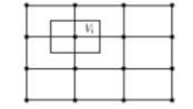 Figure 1. Volume finite method mesh element.
The resulting integral equation laws would be exactly satisfied for each element and likewise for the entire domain.
Figure 1. Volume finite method mesh element.
The resulting integral equation laws would be exactly satisfied for each element and likewise for the entire domain.
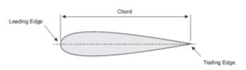 Figure 2. Hydrofoil geometry.
The characteristics of the hydrofoil are the following:
Figure 2. Hydrofoil geometry.
The characteristics of the hydrofoil are the following:
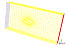 Figure 3. Mesh plot
The dimension of the entire domain was chose with regard to accuracy of the results. The dimension was limited as much as possible because of the computational cost or simulation time. The length dimension behind the ship stem is longer than that forward from the bow to get more details on the waves generated by the ship. The dimensions of the block for the simulations with a free surface were initially similar in size to the ones of the simulations without a free surface. Nevertheless, as pressure concentrations were found at the ship boundaries, they were gradually increased to better represent the fluid flow and improve the accuracy of the results.
Figure 3. Mesh plot
The dimension of the entire domain was chose with regard to accuracy of the results. The dimension was limited as much as possible because of the computational cost or simulation time. The length dimension behind the ship stem is longer than that forward from the bow to get more details on the waves generated by the ship. The dimensions of the block for the simulations with a free surface were initially similar in size to the ones of the simulations without a free surface. Nevertheless, as pressure concentrations were found at the ship boundaries, they were gradually increased to better represent the fluid flow and improve the accuracy of the results.
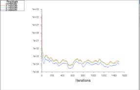 Figure 4. Convergence plot (stopped at 1495 iteration).
Simulation initial convergence was found to be considerably enhanced. It was due to the initialization procedure that it has to be careful attended. It is recommended that the primary phase is set to the lower density fluid, as in this case it was the air. The specific operating density should be set to that of the primary phase and the reference pressure location has to be set to the region of the primary phase. Also it is necessary and helpful to initialize the entire water domain with the correct hydrostatic pressure profile and to initialize both phase domains at the same velocity.
Figure 4. Convergence plot (stopped at 1495 iteration).
Simulation initial convergence was found to be considerably enhanced. It was due to the initialization procedure that it has to be careful attended. It is recommended that the primary phase is set to the lower density fluid, as in this case it was the air. The specific operating density should be set to that of the primary phase and the reference pressure location has to be set to the region of the primary phase. Also it is necessary and helpful to initialize the entire water domain with the correct hydrostatic pressure profile and to initialize both phase domains at the same velocity.
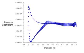 Figure 5a.CFD Pressure Coefficient.
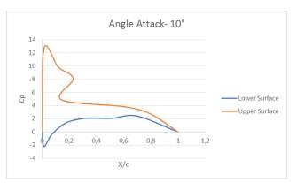 Figure 5b.Experimental Pressure Coefficient.
It was found that the main problem encountered in this study and independently was the air/water interface became considerably disrupted during the course of the simulation run. In some cases large drops of water were found to be suspended in the air in completely irregular patterns. It was necessary to repatching the appropriate part of the domain with the air phase during the course if the simulation.
The values for the pressure coefficient predicted by theoretical methods are smaller than those predicted by the CFD model. It can be conclude that the bad alignment of the struts (attack angle - 10°) in the CFD simulation can explain the relatively large values of the pressure coefficient given by the simulation.
The pressure coefficient values of CFD simulation using an angle of attack perfectly aligned are closer than those attended from theoretical experiences. Nevertheless, the CFD values of this condition do not capture the effect of the interaction between water and air.
Figure 5b.Experimental Pressure Coefficient.
It was found that the main problem encountered in this study and independently was the air/water interface became considerably disrupted during the course of the simulation run. In some cases large drops of water were found to be suspended in the air in completely irregular patterns. It was necessary to repatching the appropriate part of the domain with the air phase during the course if the simulation.
The values for the pressure coefficient predicted by theoretical methods are smaller than those predicted by the CFD model. It can be conclude that the bad alignment of the struts (attack angle - 10°) in the CFD simulation can explain the relatively large values of the pressure coefficient given by the simulation.
The pressure coefficient values of CFD simulation using an angle of attack perfectly aligned are closer than those attended from theoretical experiences. Nevertheless, the CFD values of this condition do not capture the effect of the interaction between water and air.
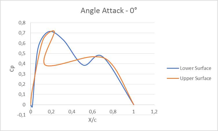
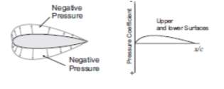 Figure 6a.Experimental results.
Figure 6a.Experimental results
Olivieri et al. [9] provide figures of the wave pattern and the wave profile along the ship at Fr=0.41 from the towing tank measurements. In figure 7, the experimental results from Olivieri et al. for the wave pattern on the free surface at Fr=0.41, and at the bottom half is the wave pattern that was found from the CFD code at the same physics work conditions. It is noticed that there is a good agreement with the CFD code results for the general form of the wave pattern from the towing tank test.
Figure 6a.Experimental results.
Figure 6a.Experimental results
Olivieri et al. [9] provide figures of the wave pattern and the wave profile along the ship at Fr=0.41 from the towing tank measurements. In figure 7, the experimental results from Olivieri et al. for the wave pattern on the free surface at Fr=0.41, and at the bottom half is the wave pattern that was found from the CFD code at the same physics work conditions. It is noticed that there is a good agreement with the CFD code results for the general form of the wave pattern from the towing tank test.
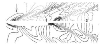 Figure 7. Experimental and CFD wave pattern at Fr=0.41.
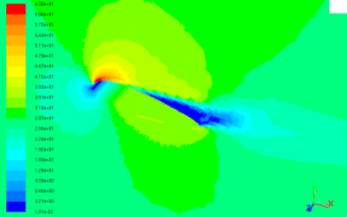 Figure 8. Dynamic Pressure Contour.
Figure.9 below shows the velocity contour at Fr=0.41. The zones with larger values of velocity (drawn with a red or closer to red colour) have a greater contribution of the frictional and pressure resistance values. It can be seen that the pressure coefficient at the tip edges receives larges values as has previously been attended.
Figure 8. Dynamic Pressure Contour.
Figure.9 below shows the velocity contour at Fr=0.41. The zones with larger values of velocity (drawn with a red or closer to red colour) have a greater contribution of the frictional and pressure resistance values. It can be seen that the pressure coefficient at the tip edges receives larges values as has previously been attended.
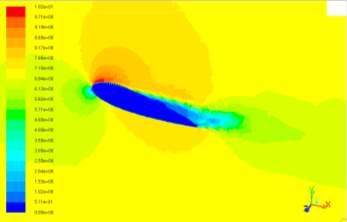 Figure 9. Velocity Contour.
In the towing tank report from literature [10] there is a photo of the bow pressure contour at Fr=0.41 The visual comparison between the CFD and the towing tank bow contour shows a similar maximum point of pressure in the geometry as shown in figure 8.
The goal of this study was to find a CFD simulation that allows compare theoretical results to these given by the theoretical values. In general the results, at the lower speeds, were not good enough. One reason of this result is that for smaller parameter values at lower speeds more accurate numerical predictions relative to the higher speeds are required to get 5% accuracy compared to the experimental data. Olivieri et al. [10] provide figures of the wave pattern and the wave profile along the ship at Fr=0.41 from the towing tank measurements. It can be seem in figure.7 the experimental results from Olivieri et al. for the wave pattern on the free surface at Fr=0.41, and at the bottom half is the wave pattern that was found from the CFD code at the same physics work conditions. It is noticed that there is a good agreement with the CFD code results for the general form of the wave pattern from the towing tank test.
Figure 9. Velocity Contour.
In the towing tank report from literature [10] there is a photo of the bow pressure contour at Fr=0.41 The visual comparison between the CFD and the towing tank bow contour shows a similar maximum point of pressure in the geometry as shown in figure 8.
The goal of this study was to find a CFD simulation that allows compare theoretical results to these given by the theoretical values. In general the results, at the lower speeds, were not good enough. One reason of this result is that for smaller parameter values at lower speeds more accurate numerical predictions relative to the higher speeds are required to get 5% accuracy compared to the experimental data. Olivieri et al. [10] provide figures of the wave pattern and the wave profile along the ship at Fr=0.41 from the towing tank measurements. It can be seem in figure.7 the experimental results from Olivieri et al. for the wave pattern on the free surface at Fr=0.41, and at the bottom half is the wave pattern that was found from the CFD code at the same physics work conditions. It is noticed that there is a good agreement with the CFD code results for the general form of the wave pattern from the towing tank test.
Keywords
Drag Reduction, Trim Optimization, Numerical Simulation, Computational Fluid Dynamics, Fuel Consumption, Ansys Fluent.1. Introduction
In the past years the computer speed has been increased exponentially and more sophisticated RANS codes have been developed. More realistic simulations are able to be performed. All these advances have been well documented in the proceedings of several international conferences on the CFD techniques applications to ship flows. These conferences have been held every year since 1990. The most famous are those in Tokyo in 1994 [2], Gothenburg in 2000 [3] and Tokyo in 2005 [4]. Remarkable information on these application of CFD codes to naval ships and submarines can be found in recent studies shown in recent proceedings of the ‘Symposium on Naval Hydrodynamics’. This symposium is sponsored by the US Office of Naval Research (ONR) and was first held in 1956. Some examples of the advancement of current specialized CFD codes for the flow simulation around naval hulls can be found in the work of Burg et al. [5] reported at the 24th Symposium on Naval Hydrodynamics. It was used in Burg’s study a three-dimensional unstructured, paralyzed CFD code named U2NCLE, developed by the Computational Simulation and Design Centre at Mississippi State University to simulate the free surface flow around a fully-appended model of a US naval ship. The results found by using this code realistically captured the turbulent flow and the vortices arising from the bulbous bow and the tips of the propulsors and rudders. Also it was found that to accurately model the propulsor rotation. Near-field wave shapes were successfully simulated by a nonlinear free surface algorithm. CFDShip-Iowa code was developed at the University of Iowa’s Institute of Hydraulic Research (IIHR) under funding provided by ONR, can be used as another example of a RANS code. This code was developed to work specifically on surface-ship interface and marine propulsor flow problems. General application in naval hydrodynamics include the prediction of resistance that include friction and pressure drag prediction, wave profiles, sea keeping using a code permitting a six-degree of freedom, and manoeuvring. Wilson et al. [6] recently compared the performance of CFDShip-Iowa code with two commercial CFD codes. Fluent, developed by Fluent Inc. and Comet, developed by CD-Adapco, in order to predict the ship generation of waves. It was found that each of the codes has different advantages and disadvantages respecting the other one, and that each code has certain specific parameters to be considered for obtaining accurate solutions of a surface ship wave fields. It was also found that commercial solvers may present and advantages when complex geometries shapes involving appendages and propulsors are being considered because of the flexibility to use unstructured create mesh contain unstructured as well as hybrid grids. Both code, Fluent and Comet, also presented the advantages of allowing solution based grid adaption techniques to provide finer grid resolution in critical regions of the grid. It can be very useful when an interface region is considered as in this case, and hence may offer a more detailed and computationally economical way to provide accurate results of the free surface prediction problems in the vicinity of surface ship hulls. Ship trim optimization operations are considered as one of most economically wise methods for both ship performance optimization and reduction of fuel consumption. There are no requirements of shape modification or puissance upgrade in such operation. It can be achieved by preparing a proper loading plan and efficient ballasting/de-ballasting process. Operationally, Trim optimization are not considered as important as other conventional power performance test procedures. Nevertheless, it was proven that trim optimization can maintain potential savings. Also, depending on the type of ship and its operation, trim optimization could result a return on investment between one to six months. These outcomes have been proven also by Hansen and Freund in 2010 [16], describing depth water influence on gains. Trim optimization test procedures can be employed in towing tank model testing or in computational fluid dynamic (CFD) simulation. Hansen and Hochkirch (2013) [17] demonstrated possible power gains by CFD tests and gave some CFD method comparisons with tests at model and full scale. Regarding the tendency of power requirement with respect to trim, both methods were found to be in reasonable agreement. A leading consultant in trim optimization as Force Technology showed possible fuel savings of up to 15% at specific work conditions. In overall fleet operation, these savings can arrive until 2% or 3%. Extensive research campaigns have been made by Force Technology to understand physical effects to reduce propulsive power. Lemb Larsen et al. in 2012 [15] presented an analysis of the origin factors in resistance and propulsive fields and the influence on power requirement. Even though resistance causes the most of power gain, overall performance can also be affected by variation in the propulsive coefficients, which could be considered as well. [15] In this paper, it was not taken in count operational constrains that should be considered in shipping, slamming or green water, strength and stability, manoeuvrability and overall safety. It was principally studied the trim optimization.2. IMO: Ship Energy Efficiency Management Plan
Recently, energy and environment issues have been studied carefully in all around the world. The objective is to promote the energy efficiency of transportation vehicles such as ships and airplanes. Nowadays, global temperature has risen about 2°C above the pre-industrial level and it is expected that it would be cause several destruction on global scale. The only way to overcome this problem is to decrease global greenhouse gas emissions. Studying future scenarios show that if preventive actions are not taken, levels of CO2 emissions from ships would be doubled by 2050. European Union (EU) and United Nations framework convention on Climate Change (UNFCCC) are working hard to get control of global emissions as shown by Kim, Hizir, Tuan, Day and Incecik, in 2017 [18]. International Maritime Organization (IMO) is currently controlling to set GHG commands for international shipping with industrial, operational, and market-based policy tools. It seems clearly IMO regulations concerning to CO2 emissions from shipping will remain to develop in coming years. Thus, fuel prices have ever been increasing and anticipated to continue growing in the future as demonstrated by Kim, Hizir, Tuan, Day and Incecik, in 2017 [18]. Several operators are promoting ship’s performance should be conduct to do constant routine maintenance and control fuel consummation efficiencies. Every day offers the opportunity to optimize speed, find the safest route and make sure the ship is sailing at the best draft and trim that is tuned to keep course safely and efficiently. These efforts are compatibles directly to the goals of recent IMO Guideline on Ship Energy Efficiency Management Plans, a framework that captures the corporate commitment to energy conservation. Most important factors that should be considered for energy conservation on ships in service are as listed below: 1. Voyage Speed Optimization 2. Weather Routing – Safe Energy Efficient Route Selection 3. Hull Roughness and Its Impact on Resistance 4. Trim/Draft Optimization In this report Trim Optimization was studied carefully to find optimal points for a simplified geometry of a ship3. Trim Optimization
Firstly, trim is defined as draught at AP and FP difference, as defined in the following expression: Trim = TA –TF In positives values trim results to the aft. Moreover, the displacement and speed keep constant when the ship is trimmed. There is not extra ballast added and power consumption varies only if resistance varies with the trim. Global goal of trim optimization is to minimize the required power at specific displacement and velocity of the ship. Physical effects of reducing propulsive power (PD) when a ship is trimmed can be caused by the hull resistance ( ) and total propulsive efficiency ( ) as shown below: PD = RT.VηD Ship speed (V) keeps constant, as said before. So, it can be concluded that the aim is to reduce the resistance and increase the total efficiency.3.1 Reduction of Resistance
According to ITTC standards, still water ship resistance is written by: RT=1/2.ρ.V2.S.CT Ship resistance changes can be a wetted surface area (S) and total resistance coefficient ( CT) function. Both parameters have to be decreased in order to get a trim gain. Wetted surface is calculated for the ship at rest, without dynamic sinkage and trim. Variation of wetted surface are caused by trim relates to the large flat stern area and it is relatively small. It can arrive to 0.5% of the even keel wetted surface and it causes that total resistance varies because of the linear proportionality. Total resistance coefficient can be achieved by reducing all parameters mentioned before. It can be described by the following expression: CT= CR+1+k.CF0+CA Allowance coefficient ( CA) keeps constants unless for ships with big variation in the draught. Friction resistance coefficient (CF0) can vary with the Reynolds number (Re) for the flow along the hull: CF0=0.075(log10Re-2)2 Where Reis the Reynolds number defined by: Re=V.Lwlν From friction resistance coefficient and Reynolds number, it can be deduced that friction resistance coefficient is a function of the water line length ( Lwl), and this relation is inversely proportional. Although water line length can vary 5% from the even keel condition, inverse proportionality results by increase or decrease propulsive power of 0.5%. This effect comparing with overall possible savings is negligible. Form factor, ( 1+k), is often kept invariable at each draught to optimize the experimental program cost in the towing tank. In practice, there is no influence giving by this factor on the resistance changes for different trimmed conditions. Residual resistance coefficient ( CR) is often the parameter most affected by the ship trim. It was seen before that residual resistance coefficient at trimmed conditions can rise up to 150% from even keel condition values. That is reflected in power requirement changes up to 20%.3.2 Increase of Total Propulsive Efficiency
Propulsive efficiency is the product result between the hull efficiency ( ηH), the open water propeller efficiency ( ηo) and the relative rotating efficiency ( ηrr). ηD=ηH.ηo.ηrr When the ship is trimmed none of these parameters are constant. Hull efficiency is a function of the thrust deduction ( t) and the effective wake fraction ( w). ηH=1-t1-w It is obvious that the thrust deduction decreases and effective wake fraction increases to achieve a gain trimming. Thrust deduction is a function of the propeller thrust ( T) and the hull resistance. t=T-RTT Also, it is known that hull resistance varies when the ship is trimmed and it causes that propeller thrust changes as the speed stays constant. Nevertheless, hull resistance is not constant. Thrust deduction changes as the trim changes and sometimes a peak, when propeller submergence decreases until arrive to a critical level, as it can be observed. The peaks localization depends on the dynamic sinkage and stern wave. Thrust deduction changings can produce values up to 15%. That means propulsive power changes up to 3%. However, the thrust deduction changes should be relatives to effective wake changes. Effective wake fraction is related to the ship velocity and the propeller inflow velocity (VA). w=V-VAV If the ship speed keeps constant, the effective wake fraction changes can only be related to the propeller inflow velocity. As mentioned before, the effective wake fraction increases for bow condition of trimming and decreases for stern condition of trimming. Wake fraction increasing for bow trims can catch up to 20% and the stern trims decreasing can rise up to 10%: Wake fraction differences can results in a power gain up to 2%. Propeller open water efficiency depends on the advancing ratio ( J), on the water inflow velocity of the propeller ( VA) and on the revolutions ( η). J=VAn.D Where Dis the propeller diameter. As concluded, propeller inflow velocity is affected by the trim. Since open water curve for the propeller efficiency is inclined for the actual ratio of advancing, with minor changes in the advance ratio result in a propulsive power changings. These changes can vary up to 2% of the even keel power demand. Relative rotating efficiency is described as the relation between the open water propeller torque coefficient (KQow) and the propeller torque coefficient behind the ship (KQship). ηrr=KQOWKQship It can be reach up to 2% from even keel condition and influencing the power requirement.4. Experimental Data
There exist extensive database for CFD validation models. Some tests were done by the Resistance Committee of the 22nd International Towing Tank Conference to create this data base [7]. The focus was on modern ship forms. Forms as tanker (KVLCC2), container ship (KCS), and surface combatant (DTMB 5415) were recommended for use. These results were shown at the workshop of Gothenburg 2000 on CFD for ship hydrodynamics [8] and other conferences. The bare hull trim results of this study were compared with the results of Olivieri et al. [9] and a combined effort between Istituto Nazionale per Studi ed Esperienze di Architettura Navale (INSEAN, Italian ship model basin [14]) and the Iowa Institute of Hydraulic Research (IIHR) to show experimental towing tank data and then compare to the CFD results. The CFD results used for compare appended model were the existing towing tank results performed by David Taylor Naval Ship Research and Development Centre [10]. This model has fixed pitch shafts and struts and is designated Model 5415-1.5. CFD Model
Computational Fluid Dynamics or CFD is a computational tool developed for studying the behaviour of the fluid flows in many different fields. It is impressive how the computer performance in this era gives us the possibility to recreate fluid flow models perfectly reals and the possibility of examining different equipment designs or compare performance under different operating conditions.5.1 Ansys Fluent Code
Fluent code is a cell centred of finite volume general resolution for CFD problems developed by Fluent, Inc. and now marketed by ANSYS, Inc. which is a provider of engineering simulation software that acquired Fluent, Inc. in 2006. Ansys Fluent has been used by the Hydrodynamics Research Group within MPD for several years to recreate problems involving submarine related flow fields. A big difference between the simulation described in this study and those reported by the Hydrodynamics Research Group is the presence of the air/water interface in the simulation. To estimate this interface there are two main approaches, either surface fitting approaches or surface capturing approaches. Ansys Fluent implemented the surface capturing approach by using VOF (Volume of Fluid) scheme for general multiphase flow modelling. This approach involves defining a volume fraction of each phase defined throughout the domain and then convecting the volume fraction of each phase with the average fluid flow. The interface between both fluids is defined from the volume fraction function for each of phase defined before in the near of the interface. The simulation of the surface ship motion not only requires maintaining a sharp interface between the water and the air phases but requires the specification of correct boundary conditions as well at the inlet and outlet of the domain for each of the phase defined in the model. One method to do this is to impose a User Defined Function to specify the total pressure and the fluid volume profile for both fluids at both inlet and outlet conditions. Another way is to use the Open Channel Boundary Condition which allows the inflow and outflow conditions to be specified from the inflow velocity and the free surface level and then the pressure and fluid volume profile can be automatically calculated. This could be simplified the simulation. Ansys Fluent offers a package of different RANS turbulence models. These include the Sparlart-Allmaras model, the k-ε model, and the k-ω model, all of which are based on the Boussinesq approximation. Boussinesq approach assumes the calculated turbulent viscosity coefficient is isotropic. Furthermore for complex flows involving streamline curvature, swirl, rotation, and rapid changes in strain rate the Boussinesq approach is not a good approximation. For these cases Ansys Fluent provides the Reynolds Stress Model (RSM), which solves the RANS equation by solving additional transport equations for each of the individual Reynolds stresses. This means that there are five additional transport equations that are solved in all three-dimensional flows and the simulation time increases substantially. In this study the simulation described involves only straight-ahead motion at minimal angles of attack. It is expected that the flow to remain largely attached to the ship surface, hence it was employed the standard k-ε turbulence model and standard wall functions for this campaign of simulations.5.2 Background
The three fundamental principles govern the physical aspects of any fluid flow are the conservation of mass, the conservation of energy and Newton’s second law. These fundamental principles are expressed in mathematical equation forms, which in a general form are integral or partial differential equations. In most cases these expressions cannot be solved analytically. Computational Fluid Dynamics (CFD) uses appropriate discretized algebraic forms to replace the integral or partial derivatives in the principles equations. These discretized algebraic forms can be solved easier. The CFD solution outcome is numbers that describe the flow filed at discrete points in time and space. Navier-Stokes equations refer to the complete system of flow equations, which solves momentum, continuity and energy equations. The complete flow system equation for the solution of an unsteady, three-dimensional, compressible, viscous flow is: Continuity Equation expression: DρDt+∇.ρ.V=0 Momentum Equation expressions: ∂(ρu)∂t+∇.ρuV=-∂p∂x+∂Txx∂x+∂Tyx∂y+∂Tzx∂z+ρfx ∂(ρv)∂t+∇.ρvV=-∂p∂y+∂Txy∂x+∂Tyy∂y+∂Tzy∂z+ρfy ∂(ρw)∂t+∇.ρwV=-∂p∂z+∂Txz∂x+∂Tyz∂y+∂Tzz∂z+ρfz Energy Equation expression: ∂∂tρe+v22+∇.ρe+v22V=ρq+∂∂xk∂T∂x+∂∂yk∂T∂y+∂∂zk∂T∂z-∂up∂x-∂vp∂y∂wp∂z+∂uTxx∂x+∂uTyx∂y+∂uTzx∂z+∂vTxy∂x+∂vTyy∂y+∂vTzy∂z+∂wTxz∂x+∂wTyz∂y+∂wTzz∂z+ρf.V Governing conservation form of equations derives from a control volume fixed in space with a fluid flow through it. Nonconservation form corresponds to the control volume moving with the fluid such that the same fluid particles are always in the same control volume. The distinction between conservation and nonconservation form was triggered by CFD development and the problem equations was more favourable to use for a given CFD application. Conservation form of the equations is more favourable for a numerical and computer programming perspective. Equation forms for an inviscid flow more known as Euler equations can be derivate from Navier-Stokes equations given above and dropping all terms corresponding to friction and thermal conduction. Navier-Stokes equations describe any fluid flow, but not all flows in the same way. The boundary conditions, and often the initial conditions, determine the particular solutions of the general governing equation for a given problem.5.3 Discretization Method
Most of CFD codes use a finite volume method of discretization, and Ansys Fluent code, used for this study, is not an exception. As that was presented above, the governing equation or Navier-Stokes equations are composed by differential equations. It represents a problem and it is necessary transform these equation into numerical equations that contain only numbers (not expression). This process produces a numerical analogue to the derivate is named numerical discretization. The discretization is made for a simple spatial domain into finite control volumes. A control volume can decompose in many elements of a mesh and, therefore, the governing equations are solved for each element of this mesh, as shown in Figure 1.
Figure 1. Volume finite method mesh element.
The resulting integral equation laws would be exactly satisfied for each element and likewise for the entire domain.
5.4 The Reynolds Averaged Navier-Stokes (RANS) Solver
Navier-Stokes equations can be solved analytically for a very small number of cases and a numerical solution is required. A numerical solution involves the governing equation discretization of motion. Once the partial differential equations are discretized it is called finite differences, but if the integral equation form is discretized it is known as finite volumes. There are some simplifying assumptions that can be made to achieve an analytical solution or to significantly reduce the computational effort demanded by the solution. This is the case when an incompressible RANS equation model is solved. Considering an incompressible flow, which is the most fluid flows assumption, the governing equation of continuity and momentum are simplified and the solution of the energy equation is no longer needed. The three velocity components are represented as a slowly varying mean velocity with a rapidly fluctuating turbulent velocity around it by the Reynolds averaging process. This method also introduced six new terms, known as Reynolds stresses. These new terms represent the increase in effective fluid velocity due to eddy turbulent existence in the flow. The turbulent models introduction serves to represent the Reynolds stresses and the underlying mean flow interactions and to close the RANS equations system. In this study the hull flow was computed using RANS equations that are becoming a standard for the numerical prediction and a viscous free surface flow analysis around ship hulls. Continuity and momentum equation, for an incompressible flow, are described by the following expression: ∇.U=0 ρU=-∇p+μ∇2U+∇.TRE+SM Where U is the averaged velocity vector, P is the averaged pressure field, μis the dynamic viscosity, SM is the momentum sources vector and TRE is the Reynold tensor stresses, computed in agreement to the K-Epsilon (k-ε) turbulent model. The Finite Volume commercial code ANSYS Fluent was used for the simulation of RANS equations on trimmed unstructured mesh.5.5 The Physics Models
5.5.1 K-Epsilon Turbulent Model
The K-Epsilon (k-ε) model is one of the most common turbulence models. The K-Epsilon turbulent model is a two-equation model known to be an eddy viscosity mode. Eddy viscosity models use the approach of a turbulent viscosity to model the Reynold stress tensor as a mean flow quantities function. In the K-Epsilon model additional transport equations are solved for the turbulent kinetic energy k and its dissipation rate ε to enable the turbulent viscosity derivation. The model transport equation for k is derived from the exact equation, while the model transport equation for ε is obtained using physical reasoning to its mathematically exact counterpart. In the procedure of the K-Epsilon model derivation, the flow is assumed as fully turbulent, and the effects of molecular viscosity are negligible. The standard K-Epsilon model is therefore valid only for fully turbulent flows.5.5.2 Eulerian Multiphase
Eulerian multiphase model is required to create and manage the two Eulerian phases of the simulations with free surface models, where a phase has a distinct physical substance. The two phases for this models are water and air, each defined to have constant density and dynamic viscosity adjusted according to the tank average temperature. This model is not required for the models that do not use free surfaces (where the inlet fluid is water), which is gain defined to have constant density adjusted to the experiment temperatures used to validate the CFD simulation. In the Eulerian Multiphase model, the different phases are treated mathematically as interpenetrating continua. As the volume phase cannot be occupied by other phase, the concept of phasic volume fraction has to be introduced. The volume fraction parameter is assumed to be a continuous function of space and time. All volume fraction addition has to be equal to the unit. The conservation equations for each phase are derivate to obtain a package of equation with similar structure for all phases. These equations are closed by giving constitutive relationships that are found from empirical information. For the case of granular flows, the application of kinetic theory is necessary.5.5.3 Volume of Fluid (VOF)
As already known the Volume of Fluid approach is used in combination with the RANS solver to determine the localization of the free surface. In this method this location is captured implicitly by determining the boundary between the water and the air long to the computational domain. An extra conservation variable is introduced and determines the proportion of water in the particular mesh cell with a value of one assigned for full and zero for empty. For the simulations where is no free surface, where there only on fluid, this model is no longer selected.5.6 Geometry and Gird
The simplified geometry was considered as a hydrofoil which is a lifting surfaces, or foil, which operates in water. It can be seem similar in appearance and purpose to an aerofoil used by airplanes.
Figure 2. Hydrofoil geometry.
The characteristics of the hydrofoil are the following:
- Hydrofoil (aerofoil adapted geometry) type: NACA0020 (Symmetrical)
- Hydrofoil Chord: 63 mm
- Hydrofoil Wing Span: 49mm
Figure 3. Mesh plot
The dimension of the entire domain was chose with regard to accuracy of the results. The dimension was limited as much as possible because of the computational cost or simulation time. The length dimension behind the ship stem is longer than that forward from the bow to get more details on the waves generated by the ship. The dimensions of the block for the simulations with a free surface were initially similar in size to the ones of the simulations without a free surface. Nevertheless, as pressure concentrations were found at the ship boundaries, they were gradually increased to better represent the fluid flow and improve the accuracy of the results.
5.6.1 Mesh Evaluation
For the mesh evaluation two scalar and dimensionless parameters were used to evaluate the generated mesh. These parameters were wall y+ and the convective Courant number. The convective Courant number is only used in implicit unsteady models, thus this parameter was used to validate the model. Boundary layer needs a high mesh resolution in the near-wall region. The normalized wall distance parameter y+ was used to check the quality of the mesh near the walls and within the boundary layer. This parameter is defined as: y+=Twρ.yν Where Twis the shear stress at the wall, ρ is the local density, y is the normal distance of the cell centroid from the wall and ν is the local kinematic viscosity. Potential errors appear with large values of y+. If it is used a high y+ wall treatment, it is generally prudent to have y+ values between 30 and 50. Moreover, there are some cells that will inevitably have a small value of y+. Most values of y+ below 100 are considered as reasonable. The lowest y+ wall treatment requires the entire mesh to have values of y+ approximately of 1 or less. In this study, the all y+ wall treatment is used because it is the most general and all values of y+ are fixed to be below 100. Convective Courant number is defined as: Convective Courant number = Vdtdx That means to evaluate the mesh with the chosen time step. Convective Courant number depends on the velocity V, the time step dt, and the interval length or length of the cells dx. This ratio of the time step and the time required for a fluid particle to travel the cell length with its local speed. For each cell this parameter is calculated and it gives an indication of how fast the fluid is going through the computational cells defined before. As it can be deduced for a finer mesh drives the Courant number at higher values, a smaller time step drives it at lower values, and a higher velocity drives it up. Implicit solvers are usually stable at maximum values in the range 10-100 locally, but with a mean value of about 1. The Courant-Friedrich-Lewy condition states that the Courant number should be less than or equal to unity. Generally, this parameter arrives to values less than 1 and it is expected to give models that run faster and with greater stability.5.7 Assumptions and Boundary Conditions
The work conditions of the simulation were the same that those in the Gothenburg 2000 workshop. The model attitude respecting to the coordinate axes was set according to the experimentally measured sinkage and trim values before creating the mesh. The coordinate system origin is located at the middle ship intersection of the water free surface and the centre plane. The open channel boundary condition was used to specify the inlet and outlet boundary condition. As has already said before, the boundary condition gives the particular solution of the general governing equation to any flow. Furthermore, these numerical solutions of the Navier-Stokes equations must give a compelling numerical representation of the proper boundary conditions. It was considered a no-slip wall boundary condition at all the walls (wall-flow and airflow and. The no-slip wall boundary condition represents the proper physical condition for a viscous flow, where the relative velocity between the boundary surface and the fluid immediately at the surface is assumed to be zero. The velocity of the flow at the surface is zero if the surface is stationary with the flow moving past it as it was defined in this case. At the inlet, it was prescribed a constant velocity that corresponds to the Froude number at which the simulation was run. The direction of the velocity that means the direction, at which the flow moves, is that of the x-axis direction. To understand, it moves perpendicular to the inlet boundary surface and toward the outlet. This inlet velocity condition is suitable for an incompressible flow. It is often utilized in combination with a pressure outlet boundary condition at the outlet flow, as it was employed in this study. The pressure outlet boundary condition is the flow outlet boundary at the outlet pressure defined. The pressure was specified to be the hydrostatic pressure of the flow with the reference pressure is the atmospheric pressure at sea level. Also, for the symmetry boundary conditions it was assumed a symmetry condition. A symmetry plane boundary condition is better used for the physical geometry with an interest and the expected pattern of the flow has mirror symmetry. A surface is defined as a symmetry plane boundary condition if it is the imaginary plane of symmetry in a simulation that would be physically symmetrical if modelled in its entirety. This solution for a symmetry plane boundary is identical to a solution that would be obtained if the mesh was replayed about the symmetry plane but in the other half of the domain. In this study, the simulations presented have an imaginary plane of symmetry where this boundary case condition was appropriate to be used. A zero-shear slip wall in viscous flows can be also modelled by a symmetry boundary condition. It was found that this condition works well and it was also used at the side, bottom and top boundaries of the simulations without a free surface. For these boundaries in the simulation with a free surface the velocity inlet boundary condition provided better performance results. The velocity imposed was the same in magnitude and direction as at inlet boundary condition. According to the real model physic, the numerical model develops a laminar regime all along the pipe and a laminar model was selected to solve the governing equations for this case. Also, the fluid was supposed incompressible, isothermal and fully developed.6. Model Simulation
An implicit steady-state cell based solution procedure was used to solve the governing equation in this study. The SIMPLE algorithm was used for the pressure-velocity coupling and a PRESTO scheme was imposed to result the pressure interpolation. A 2nd order upwind scheme was choose for the solution of the momentum equations and the modified HRIC scheme for the solution of the volume fraction equation. The relaxation factors were typically set to 0.2 and the standard K-Epsilon turbulence model with equilibrium wall functions was used to simulate turbulent flow regime. The y+ values for the wall adjacent cells over the solid geometry were in the range of 80 and 100. That allows being comfortable within the guidelines for the use of the wall function approach. Before running the simulation, it is very important to know that Ansys determines to stop the simulation taking in consideration the iteration number and convergent limit that were specified. It means that once the maximum iteration number is reached or the convergence limit is satisfied the computation is terminated. It was imposed for every calculation a convergence limit of 10E-6 for each monitor and a maximum iteration number of 1495.
Figure 4. Convergence plot (stopped at 1495 iteration).
Simulation initial convergence was found to be considerably enhanced. It was due to the initialization procedure that it has to be careful attended. It is recommended that the primary phase is set to the lower density fluid, as in this case it was the air. The specific operating density should be set to that of the primary phase and the reference pressure location has to be set to the region of the primary phase. Also it is necessary and helpful to initialize the entire water domain with the correct hydrostatic pressure profile and to initialize both phase domains at the same velocity.
6.1 Model Validation
According to experimental results which were derived from literature experimental tests, total drag coefficient is shown in figure 5. The results of series of simulation with Ansys Fluent were completely compared with the given results of experimental results. The simulation was set up to get the same situation and the same size as the ones which were utilized in theoretical experiences and good agreement could be found.
Figure 5a.CFD Pressure Coefficient.
Figure 5b.Experimental Pressure Coefficient.
It was found that the main problem encountered in this study and independently was the air/water interface became considerably disrupted during the course of the simulation run. In some cases large drops of water were found to be suspended in the air in completely irregular patterns. It was necessary to repatching the appropriate part of the domain with the air phase during the course if the simulation.
The values for the pressure coefficient predicted by theoretical methods are smaller than those predicted by the CFD model. It can be conclude that the bad alignment of the struts (attack angle - 10°) in the CFD simulation can explain the relatively large values of the pressure coefficient given by the simulation.
The pressure coefficient values of CFD simulation using an angle of attack perfectly aligned are closer than those attended from theoretical experiences. Nevertheless, the CFD values of this condition do not capture the effect of the interaction between water and air.
Figure 6a.Experimental results.
Figure 6a.Experimental results
Olivieri et al. [9] provide figures of the wave pattern and the wave profile along the ship at Fr=0.41 from the towing tank measurements. In figure 7, the experimental results from Olivieri et al. for the wave pattern on the free surface at Fr=0.41, and at the bottom half is the wave pattern that was found from the CFD code at the same physics work conditions. It is noticed that there is a good agreement with the CFD code results for the general form of the wave pattern from the towing tank test.
Figure 7. Experimental and CFD wave pattern at Fr=0.41.
Figure 8. Dynamic Pressure Contour.
Figure.9 below shows the velocity contour at Fr=0.41. The zones with larger values of velocity (drawn with a red or closer to red colour) have a greater contribution of the frictional and pressure resistance values. It can be seen that the pressure coefficient at the tip edges receives larges values as has previously been attended.
Figure 9. Velocity Contour.
In the towing tank report from literature [10] there is a photo of the bow pressure contour at Fr=0.41 The visual comparison between the CFD and the towing tank bow contour shows a similar maximum point of pressure in the geometry as shown in figure 8.
The goal of this study was to find a CFD simulation that allows compare theoretical results to these given by the theoretical values. In general the results, at the lower speeds, were not good enough. One reason of this result is that for smaller parameter values at lower speeds more accurate numerical predictions relative to the higher speeds are required to get 5% accuracy compared to the experimental data. Olivieri et al. [10] provide figures of the wave pattern and the wave profile along the ship at Fr=0.41 from the towing tank measurements. It can be seem in figure.7 the experimental results from Olivieri et al. for the wave pattern on the free surface at Fr=0.41, and at the bottom half is the wave pattern that was found from the CFD code at the same physics work conditions. It is noticed that there is a good agreement with the CFD code results for the general form of the wave pattern from the towing tank test.
7. Conclusion
The present study presents how possible it is to numerically create a functionally model of a container ship from a simplified geometry. This approximation gives a pretty good estimation of the results attended from theoretical experiences. Some of the scientific papers related to this problem consider the flow as unsteady flow, attached to a cavitation model at high ship velocities. Using that large eddy simulation model as turbulence model could also capture the free surface effect on the hydrofoil as the hydrofoil position during service is around to the surface water. Nevertheless, it was proved that using a K-Epsilon model and considering the flow as two dimensional and fully turbulent flow gives well estimation of the physical working. Numerical approach was used to calculate the free-surface flow around a simplified geometry of a DTMB 5415-1 naval ship model. The simulations were performed using hexahedral mesh after doing some mesh sensibility tests. The results given by the simulation show that this numerical approach is able to accurately simulate the total pressure coefficient, near-field wave shapes, and the pressure and velocity field in the propeller plane. Using Ansys Fluent it can be found that the software is particularly sensitive to the attack angle of the grid respect to the free surface water line in simulation of this kind. This can represent a problem, but I can be solved by re-meshing the geometry for each individual sinkage and trim calculation. The pressure coefficient calculated on the simulation within an attack angle null was found agree with the experimental value to within 8.3%. The simulated velocity and pressure contour shapes along the surface of the ship were found to be in good qualitative agreement to those of experimental profiles. Regarding the possible power saving it should be conclude that for medium speed ranges the results are not changing, while for the angle of attack deviation reach from 0.7 up to 14. Thus, this could be a recommended for better power saving prediction in the speed range considered. Therefore, the predicted power saving are generally lower, but it exhibit a good approximation of real experiences. The above results are encouraging and indicate that Ansys Fluent code is a viable tool and it could be considered for use in more demanding real problems.8. Recommendation for Future Work
This study was focused on optimizing trim of ship simplified geometry. Next step would be to simulate a more realistic geometry to compare the results obtained in this study. In the direct power saving, that could be considered to predict power levels a wake scale effect and correlation allowance coefficient. References- M. Reichel, A. Minchev & N.L. Larsen, ‘’Trim Optimisation - Theory and Practice’’, FORCE Technology, Kgs. Lyngby, Denmark, 2014.
- Kodama, Y., Takeshi, H., Hinatsu, M., Hino, T., Uto, S., Hirata, N. and Murashige, S., “Proceedings of the 1994 CFD Workshop”, Ship Research Institute, Japan, 1994.
- Larsson, L., Stern, F. and Bertram, V., “Benchmarking of Computational Fluid Dynamics for Ship Flows: The Gothenburg 2000 Workshop”, Journal of Ship Research, 47, No.1, pp. 63-81, March 2003.
- Hino, T. (ed.), “Proceedings of the CFD Workshop Tokyo 2005”, Tokyo, Japan, 2005.
- Burg, C.O.E, Sreenivas, K., Hyams, D.G. and Mitchell, B., “Unstructured Nonlinear Free Surface Simulations for the Fully-Appended DTMB Model 5415 Series Hull Including Rotating Propulsors”, Proceedings of the 24th Symposium on Naval Hydrodynamics, Fukuoka, Japan, 8-13 July, 2002.
- Wilson, W., Fu, T.C., Fullarton, A. and Gorski, J., “The Measured and Predicted Wave Field of Model 5365: An Evaluation of Current CFD Capability”, presented at the 26th Symposium on Naval Hydrodynamics, Rome, Italy, 17-22 September, 2006.
- ITTC, 1999, "Report of the Resistance Committee," Proceedings International Towing Tank Conference, Seoul, Korea & Shanghai, China, 5-11 September.
- G2K 2000, http://www.iihr.uiowa.edu/gothenburg2000.
- Stern, F., Longo, J., Penna, R., Olivieri, A., Ratcliffe, T., and Coleman H.: International Collaboration on Benchmark CFD Validation Data for Surface Combatant DTMB Model 5415, Twenty-third Symposium on Naval Hydrodynamics, 401-420, Val de Reuil 2000.
- Olivieri, A., Pistani, F., Avanzini, A., Stern, F., and Penna, R.: Towing tank experiments of resistance,sinkage and trim, boundary layer, wake, and free surface flow around a naval combatant INSEAN 2340 model, IIHR Technical Report No. 421, 2001.
- Heydarian A. and Pengfei Liu, ‘’Ship Trim Optimization for the Reduction of Fuel Consumption’’, 2014.
- D.A. Jones and D.B. Clarke, ‘’ Fluent Code Simulation of Flow around a Naval Hull: the DTMB 5415’’, Maritime Platforms Division Defence Science and Technology Organisation, Victoria, 2010.
- https://www.slideshare.net/AhmedGamal155/hydrofoil-ship-simulation-using-ansys-fluent , (Hydrofoil CFD Workshop)
- INSEAN Research Institute - www.insean.cnr.it
- Lemb Larsen N., Simonsen C.D., Klimt Nielsen C., Råe Holm C. (2012), Understanding the physics of trim, 9th annual Green Ship Technology Conference,Copenhagen, Denmark
- Hansen H., Freund M. (2010), Assistance Tools for Operational Fuel Efficiency, 9th International Conference on Computer and IT Applications in the Maritime Industries, COMPIT 2010, Gubio, Italy
- Hansen H., Hochkirch K. (2013), Lean ECO‐Assistant Production for Trim Optimisation, 11th International Conference on Computer and IT Applications in the Maritime Industries, COMPIT 2013, Cortona, Italy
- Kim, Mingyu and Hizir, Olgun and Turan, Osman and Day, Sandy and Incecik, Atilla (2017) Estimation of added resistance and ship speed loss in a seaway. Ocean Engineering, 141. pp. 465-476. ISSN 0029-8018
Cite This Work
To export a reference to this article please select a referencing stye below:
Reference Copied to Clipboard.
Reference Copied to Clipboard.
Reference Copied to Clipboard.
Reference Copied to Clipboard.
Reference Copied to Clipboard.
Reference Copied to Clipboard.
Reference Copied to Clipboard.
Related Services
View all


Related Content
All TagsContent relating to: "Maritime"
Maritime is something relating to the seas and oceans. The term is commonly used in nautical and seaborne trade matters. Not to be confused with “marine” which relates specifically to the seas, oceans and the life within them.
Related Articles

DMCA / Removal Request
If you are the original writer of this dissertation and no longer wish to have your work published on the UKDiss.com website then please: