Vertical Mixing Of Lakes Around The World

Abstract

This report explores the relationship between the rate of vertical mixing in stratified lakes across the world and the corresponding lake profile and location. The importance of mixing is explored and its relationship with drinking water quality and how it may be impacted by climate change. The vertical eddy diffusivity coefficient, K_Z, was extracted from literature and compared with the volume, surface area, maximum depth, average depth, elevation and latitude of 14 data sets with a PCA analysis using the metalimnion eddy diffusivity value. The results show significant positive correlation between the lake size and the eddy diffusivity, and a second positive correlation between the eddy diffusivity and the elevation. This research will contribute to further modelling of the impacts of climate change.

Table of Contents

Abstract

Acknowledgements

1.0 List of Figures

2.0 List of Tables

3.0 List of Symbols

4.0 List of Abbreviations:

5.0 Introduction

5.1 Our Water is Under Threat

5.2 Aims of this dissertation

5.3 Terminology

6.0 Literature Review

6.1 The Importance of Mixing

6.2 What are internal waves?

6.4 The impact of climate change on stratified Lakes

6.5 Rising Water Temperatures

6.6 Oxygen Depletion

6.7 Eutrophication

6.8 The consequences of oxygen depletion

6.9 Effect on Drinking Water Quality

6.10 Conclusion

7.0 Experimental Design

7.1 Extracting the Eddy Diffusivity

7.1.1 Case Study Paper: Turbulent mixing induced by nonlinear waves in Mono Lake, California

7.1.2 Using graphically represented data to estimate KZ

7.1.3 Other Papers

7.1.3 Determining eddy diffusivity with the Lake Number

7.2 Lake Profile Data Collection

7.3 Principle Component Analysis

8.0 Results and Analysis

8.1 Variables against Eddy Diffusivity

8.2 PCA (Principle Component Analysis)

9.0 Discussion

9.1 Table of results

9.2 Discrepancy in eddy diffusivity values

9.3 PCA

10.0 Limitations of study

10.0 Conclusion

Bibliography

Appendix

1.0   List of Figures

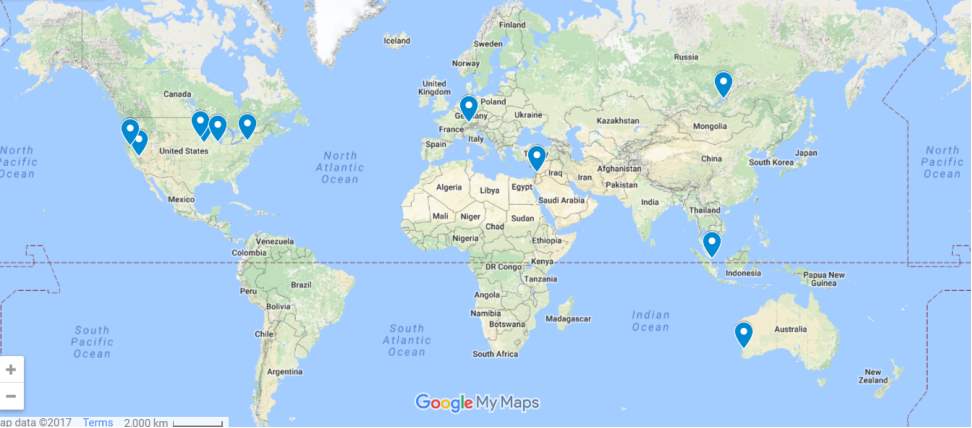
Figure 1 – Map of Lakes Studied, (Google Maps, 2017)

Figure 2 – A diagram of a stratified lake

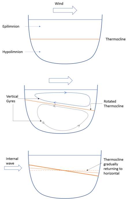
Figure 3 – Schematic of internal waves

Figure 4 – Eddy Diffusivity Data provided for Mono Lake California, (McIntyre, et al., 2009)

Figure 5 – Temperature and Eddy Diffusivity profile for location C in Mono Lake, California, (McIntyre, et al., 2009)

Figure 6 – Temperature and eddy diffusivity profile of Cayuga Lake, (Dorostkar & Boegman, 2013)

Figure 7 – Lake Constance Lake Number plotted against time, (Yeates & Imberger, 2003)

Figure 8 – The comparison of eddy diffusivity and the lake volume.

Figure 9 – The comparison of eddy diffusivity and the surface area of the lake.

Figure 10 – The comparison of eddy diffusivity and the maximum depth of the lake.

Figure 11 – The comparison of eddy diffusivity and the average depth of the lake.

Figure 12 – The comparison of eddy diffusivity and the elevation of the lake.

Figure 13 – The comparison of eddy diffusivity and the absolute latitude of the lake.

Figure 14 – Scree Plot of PCA analysis, showing the percentage of variance attributed to each principle component analysis and the associated eigenvalue

Figure 15 – Correlation Circle, showing how the variables are linked with the first two principle components

2.0   List of Tables

Table 1 – Table of Results

Table 2 – Eigenvalue table showing the variability attributed to each principle component

Table 3 – Contribution of variables to each significant Principle Component

Table 4 References correlating to the data found for the table of results

3.0 List of Symbols

4.0 List of Abbreviations:

PCA – Principle Component Analysis

K_Z – Vertical Eddy Diffusivity coefficient

K_M – Molecular Diffusivity of heat

L_N – Lake Number

5.0           Introduction

5.1 Our Water is Under Threat

Many people in the developed world take for granted that turning on the tap will provide unlimited and safe drinking water necessary for a wide range of everyday tasks. The average daily use of water per person in the U.S. is 80-100 gallons (Perlman, 2016). Unfortunately, most of the earth’s water is saline, which requires vast amounts of energy input to become of drinking water quality. Population growth is continuing at an exponential rate and water supplies are not distributed evenly, the Intergovernmental Panel on Climate Change (IPCC) currently predicts that 60% of the world’s population will not have access to enough drinking water by 2050 (European Commission, 2015). The supply of accessible, non-saline water available often only from freshwater lakes and through expensive infrastructure projects (see Niger Dam) is a precious resource that needs to be protected in a sustainable manner for future generations. Additionally, the climate is changing at ever quicker rates and the impact of the increase in global temperature and extreme weather events may have on the world’s freshwater resources are relatively unknown.

5.2 Aims of this dissertation

This paper aims to explore the changes that will occur to lakes and reservoirs that currently contain much of the supply of freshwater over the next century. It will first define the relevant terms used to describe these changes by explaining the importance of mixing particularly in seasonally stratified lakes, the function of internal waves, and define key terminology used in much of the literature.

It comprises a literature review that summarises much of the current research into freshwater lakes, especially that which pertains to increased temperature and the consequences of increased stratification strength. This establishes the purpose of this dissertation to understand the relationship between the rate of vertical mixing in lakes across the world and their location and profile by collating much of the observation data presented in the scientific literature.

The lakes included in this study have been highlighted on the map in Figure 1. An analysis had been conducted of the statistical relationships between observed data of the vertical eddy diffusivity coefficient of a range of lakes and their corresponding lake profile and location. Establishing a known relationship between the rate of mixing and lake location or lake profile could lead to a greater awareness of the possible warning signs to the dangers of enhanced stratification. Further research understanding the impacts of climate change (particularly global warming) on the lakes studied here could use this dissertation’s results to model global implications on freshwater sources. This may enable more accurate modelling of how lakes around the world would respond to climate change and be used to create frameworks for sustainable management practices to protect the global supply of freshwater.

Figure 1 – Map of Lakes Studied, (Google Maps, 2017)

5.3 Terminology

Within this this dissertation several terms will be used when describing the vertical mixing of lakes.

Lake Stratification: Stratification is a process in which defined layers are created in a large, often still, water body. The process of stratification within a deep-water body occurs because of a difference in water density. This can be caused by differing salinity, or by a significant temperature difference. Warm water has a lower density (as density is shown to decrease with increased temperature) and will rise to the surface. Lakes are heated from the surface, through solar radiation, this means the top, warm layer stays at the surface rather than mixing with the bottom layers.

Stratified lakes are categorized into three distinct layers Epilimnion, Metalimnion and Hypolimnion, as can be seen in Figure 2.

Epilimnion: The surface layer of the lake which has the highest temperature and greatest turbulence.

Hypolimnion: The bottom layer of the lake. This layer is the coolest, with the highest density and has the lowest rate of mixing.

Metalimnion: The middle layer of the lake that exhibits the greatest temperature differential across its depth profile.

Thermocline: This is the depth at which the temperature over depth gradient is the greatest, as seen in Figure XX.

Boundary Layers: The layers at the edges of the lake, that are adjacent to the bank. The boundary layer is typically more turbulent than the lake interior at the same depth, this is due to the reflected internal waves and from internal currents caused by seismic, wind or atmospheric differences, commonly known as seiches (Wain, et al., 2013).

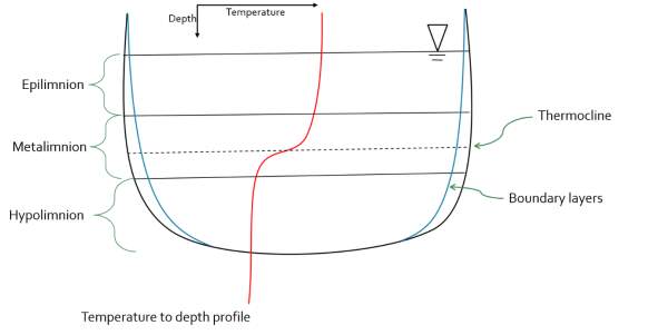
Figure 2 – A diagram of a stratified lake

 

Seasonal Stratification: Many lakes are only stratified during the summer months when temperatures are high enough to generate significant temperature differences in the water body. This is called seasonal stratification, it can also take place in large, slow moving rivers. During autumn when the temperature levels drop again there is sufficient mixing to remove the defined layers that had been created.

Eddy Diffusion: The process of diffusion in water due to turbulent, or eddy, motion.

Eddy Diffusivity Coefficient (K_Z): The eddy diffusivity coefficient is the enhanced rate of diffusion (above molecular diffusion) due to turbulent, or eddy, motion.

Benthic: Organisms or processes that occur at the bottom level of a water body, often in the substrate.

Internal Waves: (See 1.4) Internal waves are a driving force for mixing deeper within a lake. As explained by Fischer, wind stress forcing the epilimnion to move in the direction of the wind, with the water surface layer remaining constant, the hypolimnion counters this flow moving in the opposite direction. (Fischer, et al., 1979)

Gyre: The cyclic movement of fluid, this happens in oceans due to the Coriolis effect. It can also happen vertically due to shear.

Seiching currents: Waves driven by atmospheric or seismic disturbances.

Lake Number: A ratio representing the strength of stratification over the strength of the wind destabilising the stratified lake.

6.0 Literature Review

This dissertation will explore the relationship between the eddy diffusivity coefficient, the lake profile and lake location. The eddy diffusion inherently is a measure of the rate of mixing within a stratified lake. The following literature review explores the current research into this field.

6.1 The Importance of Mixing

The importance of vertical mixing in lakes cannot be overestimated. Mixing is essential to evenly distributing dissolved substances, including oxygen and nutrients throughout the waters depth (Wain & Rehmann, 2010). This dispersion is fundamental to sustain a healthy and diverse ecosystem. Mixing also prevents the isolation of chemical and biological compounds that have potential to be damaging to human and aquatic life, such as heavy metals or toxic algae.

In non-stratified lakes, the currents are normally sufficient to provide the required mixing. In a stratified lake, the separation of layers inhibits mixing and turbulence from internal waves and intrusions from the turbulent boundary layer are key sources of mixing. Internal wave dynamics are very complicated and progress in understanding this has largely been from empirical results (Wüest & Lorke, 2003).

Research into how boundary mixing affects the movement of nutrients and oxygen has been conducted through experiments with dye and measuring the intrusions (Wain & Rehmann, 2010). These intrusions are greater than the mixing in the interior of the lake and therefore assumed to be a result of the interaction between seiching currents and the boundary. The Ada Hayden Lake is one of the lakes used in this dissertation’s research, though a lack of eddy diffusivity data for a wide range of lakes in the boundary layer, led to the boundary layers not being included in this study. (Wain & Rehmann, 2010) impresses the importance of gaining a better understanding of lake mixing. This is because mixing recirculates key nutrients and oxygen which is key to a healthy eco system and managing water quality.

This dissertation studies the relationship between the rate of vertical mixing and the properties of the lake profile and location.

6.2 What are internal waves?

Internal waves, also known as gravity waves, are largely driven by the wind stress at the surface layer. Around 10% of this mechanical wind energy penetrates the surface boundary layer into the depth of the lake and this energy is then transferred to internal wave motions (Wüest & Lorke, 2003).

The epilimnion is first pushed in the direction of the wind as demonstrated in figure AA, creating an asymmetrical depth across the water profile. The increased depth of the epilimnion layer on one side of the lake in turn causes an increase in pressure exerted on the hypolimnion, across the thermocline. This causes the hypolimnion layer to be pushed towards the opposing side of the lake as shown in Figure 3, A, resulting in the thermocline existing at an angle. Here, the epilimnion is forced into the formation of a vertical gyre, as shown in Figure 3 B, above the thermocline and in the hypolimnion an opposing vertical gyre is also formed beneath the thermocline producing shear against one another. (Fischer, et al., 1979). In this arrangement, due to the difference in densities of the layers, the weight of the left-hand side one is now greater than on the right as the hypolimnion (most dense layer) forms a greater percentage of the water profile and, conversely, the epilimnion (less dense layer) forms a smaller part of the water profile. Over time the hypolimnion layer pushes back to be horizontal level again, due to gravity, creating a flowing movement through the water that is referred to as an internal wave. Figure 3 C shows how the thermocline returns to horizontal.

Whilst internal waves cannot be seen at the surface level, in oceans they can be as tall as sky scrapers. However, in the freshwater lakes that this study is concerned with, they are smaller, simply due to the size of water body. They are the cause of several different phenomenon including ‘dead water,’ an event that occurs when ships experience excessive drag in seemingly calm waters (Pannard, et al., 2011) and more importantly for this paper, play a crucial role in water mixing when lakes are stratified, especially important for the distribution of phytoplankton in the summer months.

6.4 The impact of climate change on stratified Lakes

Any rise in strength of stratification inevitably means a reduction in the rate, and magnitude, of vertical mixing between stratified layers. This leads to growing concentrations of oxygen and nutrients in certain areas of the lake rather than an even distribution. Increased strength of stratification can lead to many negative consequences for lake biodiversity, the most notable being anoxia and eutrophication. Both processes can be part of a positive feedback mechanism prompting further reductions in dissolved oxygen and release of carbon dioxide into the air, and further reductions in biodiversity.

The impact of climate change on specific lakes has been studied but the global impact on freshwater resources is not yet known. The research in this dissertation will show the correlation of mixing between lakes; this will enable future predictions to be drawn on lakes that have not been studied.

6.5 Rising Water Temperatures

Studies in Lake Zurich, Switzerland, have recorded a significant change in the temperature profile of the lake in recent times. In the period between the 1950s and 1990s the lake temperature has been measured to have increased in the top 20m of the lake by 0.24K per decade and decreased in temperature at depths greater than 20m by 0.13K per decade (Livingsone, 2003). This shows that within recent history of northern hemisphere freshwater lakes there has been an increased temperature difference between the epilimnion and hypolimnion. This is evidence of an increase in the strength of the stratification. As a seasonally stratified lake, stratification has also been observed to last an extra 2-3 weeks in 1990 than in 1950 (Livingsone, 2003). Research in Lake Tahoe, California, a relatively shallow lake, also shows an annual increase in summer lake temperature. It was observed that between 1972 and 1998 there was an annual increase of 0.015 ◦C yr⁻¹, again evidence for an increase in the thermal stability of the lake (Coats, 2006).

Whilst the research done in Lake Tahoe and Lake Zurich in the above papers clarifies how the increase in temperature has already impacted the lake profile, it is limited in its usefulness to this paper. One limitation of this research is that there is no forecast of the possible future changes to the Lakes due to climate change. However, the conclusions are helpful as they demonstrate the warming effect that is already taking place, and observe the increased stratification that has been caused by this. There may be some observational errors in data collection that would also limit the usefulness of these papers, particularly in the earlier parts of this study when less reliable and accurate equipment may have been used.

6.6 Oxygen Depletion

A consequence of the changing climate that may affect lakes is oxygen depletion, or the overall level of dissolved oxygen within the lake decreasing. This can partly be assumed to be associated with the reduction of oxygen in the air. The rate of atmospheric oxygen depletion is very small, a reduction of 19 O₂ molecules per year, nonetheless the continued depletion could cause problems for our freshwater resources (Scripps O2 Programme, 2016). Blelham Tarn in the UK has measured oxygen depletion; the reduction in dissolved oxygen shows a strong correlation to the time of thermal stratification. Blelham Tarn has become stratified earlier in the year and the stratification season lasted longer than before, this has led to an increase in the stratification period of 38 ± 8 days over the 41 years. (Foley, et al., 2011). This is likely a result of the increased temperature and associated effects observed in Lake Zurich and Lake Tahoe. With a stronger stratification profile and less oxygen in the lake overall, the amount of oxygen in the hypolimnion is rapidly decreasing. The stronger stratification for a greater time frame means that internal waves are becoming a vital source of mixing. Further research into the eddy diffusion in seasonally stratified lakes is critical.

6.7 Eutrophication

Eutrophication is caused by excessive nutrients in a lake, commonly nitrogen and phosphorus. This allows the fast and excessive growth of plants and algae that were previously limited by the lack of nitrogen available. The immediate impact of such blooms is the blocking of sunlight, and, by extension, prevention of photosynthesis for phytoplankton that exist in the lower layers of the freshwater lake. Additionally, once these blooms die off and sink to the bottom they are digested by benthic bacteria that further consumes oxygen present in the in the hypolimnion.

The effects of high concentrations of phosphorus can be shown through the research of 71 Danish lakes. The lakes with high concentrations of phosphorus had reduced species richness and the body weight of fish was lower, particularly in zooplankton (Jeppesen, et al., 2000). Once eutrophication has occurred, it is very hard to return the ecosystem to full health.

Eutrophication can occur in a range of water bodies, lakes and slow moving rivers or canals. This can be a problem in the urban environment as well as in rural locations. For example, current research is being carried out in Manchester Ship Canal with the aim of ecological restoration, this requires oxygenation. (Williams, et al., 2010)

6.8 The consequences of oxygen depletion

Oxygen depletion can cause dead zones or areas of the lake which do not have enough oxygen to support life. This means the fish suffocate if they do not manage to leave the dead zone. It can be caused by anthropogenic eutrophication water pollution through excessive plant nutrients, this is often attributed to fertilizers used in agriculture. The introduction of nitrogen and phosphorus rich fertilizers to a freshwater lake allows excessive algae growth.

Research shows that oxygen depletion can be accelerated by changing temperature. Lake Erie, one of the five great lakes in North America, is crucial to the tourism and fishing industry of the local area. It has been of interest to the scientific community due to an area of very low oxygen that was discovered in the 1960s when the understanding of human impacts on both climate and limnology was much more limited than it is today. At that time, change in lake profile at certain depths was predominately measured by the change in population of a particular species. Evidence used to support the change in ecosystem included the decline of the Hexagenia mayfly from 139 /m³ in 1930 to below 1/m³ in 1961 (Carr & Hiltunen, 1965). It is widely accepted that the dissolved oxygen depletion of Lake Erie can be attributed to industrial waste, agricultural waste, and the pollution of sewage treatment plants. Phosphorus, and the related eutrophication, was attributed as a leading cause of the oxygen depletion (GLIN, n.d.).

Future predictions of global warmings impact on Lake Erie have been modelled. The doubling of atmospheric CO₂ is expected to have a significant impact on the water quality. The dissolved oxygen is predicted to reduce by 1mg/L in the epilimnion and 1-2mg/L in the hypolimnion in the lake interior (Blumberg & Toro, 1990). The modelled decline was hypothesised to be due to the warmer lake temperatures, which would drive an increase in the rate of bacterial activity particularly in the lowest parts of the lake, namely the hypolimnion and the sediment. This would be sufficient to cause significantly lower dissolved oxygen concentrations. In contrast to the research previously mentioned, which attributed reduction in dissolved oxygen to stronger stratification; this research determined the decline of dissolved oxygen was independent to the thermocline depth. (Blumberg & Toro, 1990).

Blumberg and Toro hypothesise that the position of the thermocline will have little influence on the levels of dissolved oxygen in the water. This contrasts with the research done in Lake Zurich (Livingsone, 2003). The model that has been designed to predict of potential changes in Lake Erie’s profile has many assumptions, this creates many potential margins of error. Due to the changing climate, there may be a future global trend for oxygen depletion in other water bodies also associated with a rise in CO₂ levels. Many climate change models forecast an outgassing of oxygen from the ocean (Matear, et al., 2000), and it can be argued that lakes and reservoirs also play a large role in regulating both regional and global oxygen and carbon dioxide levels (Lars J. Tranvik, 2009).

6.9 Effect on Drinking Water Quality

As we can see the increase in global air temperatures will increase the thermal stratification of lakes, reducing the mixing of lakes. It is important for lakes to mix to keep the oxygen levels throughout the lake moderated. Lack of oxygen in lakes results in a higher level of metals dissolved in the water. Untreated, it has the potential to contain toxic levels of iron or manganese ions. These can lead to severe health problems to new-born babies and young children including but not limited to brain damage, and damage to the central nervous system and red blood cells (Gautam, et al., 2014). In the developed world, the water treatment process manages the metal ion levels so they do not pose this risk. However, the greater the ions in the water source, the higher the energy required to reduce them. This in turn rises the cost, and increases the carbon emission of the process. After treatment, a safe, but high level of metal ions may still be present and cause the water to discolour or taste unappetizing and therefore make it very unappealing for public consumption.

6.10 Conclusion

Research into mixing so far is focused on regional cases. Further research has also been done to the origins of mixing in stratified lakes, internal waves and boundary intrusions. Limited conclusions can be drawn on lakes with little research because there are no comparative studies. This dissertation researches the potential of a relationship between lakes and the rate of mixing through the eddy diffusivity coefficient. Through this study, future predictions can draw on other data from other lakes with similar critical lake properties. Understanding the relationship between rate of mixing and lake properties could prove invaluable in the fight to sustain our freshwater resources in the ever-changing climate.

7.0 Experimental Design

Data used for this research has been extracted from research studies available in literature. Consequently, 10 sources covering 14 data sets over 11 lakes were used, each presenting data slightly differently. The first step was to establish whether the data allowed the vertical eddy diffusivity coefficient to be established. Some journals found during research could not be used, these include reasons such as:  not reporting the vertical eddy diffusivity coefficient values, for example: “Seasonal evolution of the basin-scale internal wave field in a large stratified lake” (Antenucci, et al., 2000), lakes that were stratified due to salinity and therefore fell outside the width of this research. There were also lakes with only the boundary eddy diffusivity data shown, as there was not sufficient boundary layer data on a range of lakes it has not been included in this research.

7.1 Extracting the Eddy Diffusivity

The methodology differed slightly depending on how the data was provided in each article. This section will go into more detail on a typical example of extracting the eddy diffusivity coefficients for each layer of the lake. This paper uses a typical notation for the vertical eddy diffusivity coefficient as: K_Z.

7.1.1 Case Study Paper: Turbulent mixing induced by nonlinear waves in Mono Lake, California

Figure 4 shows graphs of the eddy diffusivity, measured in Mono Lake, (McIntyre, et al., 2009). The four different charts: A, B, C and D represent four different locations within the Lake. The two temperature lines for each graph show that they were measured on two different days, for example in graph A the solid line was taken on the 106^th day in the calendar year and the dashed 112^th day of the calendar year. The eddy diffusivity was measured every day between the temperature readings, and a 95% confidence interval has been shown with the rectangular box section at the end of the bar graph, the smaller the box the more concentrated the results were, for example the depth of 12m in locations C and D had the widest spread of results, which we can deduce because the box is bigger, in comparison the values for the epilimnion in location A had a small range of results. 

Figure 4 – Eddy Diffusivity Data provided for Mono Lake California, (McIntyre, et al., 2009)

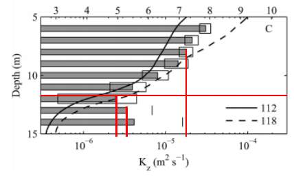
7.1.2 Using graphically represented data to estimate K_Z

A step by step process below shows how the data was extracted in a typical case study, refer to Figure 5.

1. First the depth at which the temperature gradient was at its shallowest was determined. This depth is the location of the thermocline. The Metalimnion depth is either side of the thermocline.
   Thermocline Depth = 12 m, Metalimnion Depth = 11-13 m.

2. Then at the depth of the thermocline, the eddy diffusivity coefficient is read off the graph.
   K_Z at Metalimnion = 2.3 x 10^-6 m²s^-1
3. The average Epilimnion depth can be estimated to be half way between the surface of the lake and the thermocline.
   Average Epilimnion Depth = 6 m

K_Z at Epilimnion = 1.8 x 10^-5 m²s^-1

4. The average Hypolimnion depth can be estimated to be half way between the bottom of the lake and the thermocline.
   Average Hypolimnion Depth = 14 m
   K_Z at Hypolimnion = 3.2 x 10^-6 m²s^-1

Figure 5 – Temperature and Eddy Diffusivity profile for location C in Mono Lake, California, (McIntyre, et al., 2009)

7.1.3 Other Papers

When several locations within a lake had been measured, an average of these has been used. An alternative would have been to use each of the values however it was decided it was more representative to consider the mean of the whole lake to reduce peak errors that may occur if there are some anomalies in the data. As the paper is comparing different lake profiles, an overview of each lake was more appropriate than detailed information for different locations within a lake. Locations that were deemed to be too close to the boundary of a lake were omitted, this is because the boundary layer of a lake behaves differently, with a greater turbulence.

Each paper has presented data differently and has been extracted accordingly. As can be seen below in Figure 6 used a colour plot with isotherms on a chart with mapped eddy diffusivity, in this case the depth where the isotherm lines were closely packed was taken to be the thermocline and the eddy diffusivity reported only to the nearest factor of 10.

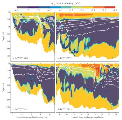
Figure 6 – Temperature and eddy diffusivity profile of Cayuga Lake, (Dorostkar & Boegman, 2013)

7.1.3 Determining eddy diffusivity with the Lake Number

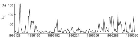
“Pseudo two-dimensional simulations of internal and boundary fluxes in stratified lakes and reservoirs” (Yeates & Imberger, 2003) used data from Lake Kineret to determine a relationship between the K_Z at the metalimnion and the Lake Number, Lake Number is the ratio between the strength of the stratification and the strength of the wind.

For research in this dissertation, this relationship has been assumed true.

Yeates, 2003, also reported the Lake number for Lakes: Constance, Mono Lake, Kinneret, Crystal Lake and the Mundaring Reservoir. Figure XX shows how the lake number was reported, through the example of Lake Constance. The Lake Number was plotted against time, to determine the average Lake Number, the plot was digitized. This involved tracing the pdf image from the paper, with a tool (http://plotdigitizer.sourceforge.net/) that converts the graph into a data file which can be read by excel. This data file has the xy coordinates of each reading, and the mean value of the Lake Number can be determined. Given the nature of the assumptions underpinning this analysis the eddy diffusivity coefficients determined have been considered only to the nearest factor of 10.

7.2 Lake Profile Data Collection

The variables considered were: Volume, Surface Area, Maximum Depth, Average Depth, Elevation and Latitude. The variables that weren’t reported in the journals with the associated eddy diffusivity, were drawn from a mix of scientific literature and online sources. These have been referenced in the results section, Table 1. Some lakes the volume has not been reported: (Castle Lake, Lake Ames, West Okoboji Lake, Kranji Reservoir, Mundaring Reservoir), in this case the volume has been determined by equation 1. The average depth of Mundaring Reservoir has also not been reported, a sensible estimation was assumed based on 85% of the maximum depth.

Volume=Surface Area ×Average Depth                                                         (1)

7.3 Principle Component Analysis

A PCA was chosen to compare the data because several variables are changing at once. Eddy diffusivity has been plotted against each variable separately for interest, see figures 34-97, but they have limited use in determining if there is a correlation between the data as there is more than one variable. PCA considers the greatest degree of variability (principle component 1) across the study and the variables that influence this, before considering the second greatest variability, etc. This PCA was carried out by using an excel extension, XLSTAT.

There are several advantage of using a PCA over a Pearson’s correlation, for example a PCA compares data with variables that change simultaneously, while a Pearson’s correlation only looks one variable at a time, for example the eddy diffusivity against the volume and not does consider the impact of the other items varying, Pearson’s correlation is good to use for lab experiments when only one variable has been adjusted, however it is less helpful in field situations with many impacting properties. Another limitation of the Pearson’s correlation is that to show a relationship, in this case the outliers need to be eliminated, with only 14 data sets to begin with, reducing the data further is not ideal, PCA allows you to keep all the data.

As the results for the hypolimnion and epilimnion were missing for some of the lakes, a PCA was conducted only on the metalimnion values. An alternative would have been to conduct three PCAs on each layer, however the lack of data means that the PCA would not have been reliable for the epilimnion or hypolimnion layers (with only 7 and 9 data sets accordingly). Combining the three data sets to create an average eddy diffusivity value for each lake was considered, however this would not have been representative of the true average of the lake. Hypolimnion and epilimnion eddy diffusivities are typically higher than at the metalimnion, so the lakes with only the metalimnion values reported would have been reported to have a lower average eddy diffusivity than the true value.

8.0 Results and Analysis

The Results from the data collection can be seen in Table 1. Lakes which have had multiple reports on them are distinguished with (1) and (2). The references for the data in this collection can be seen in the appendix. As shown in the table there was not data for all the eddy diffusivity values for the hypolimnion and epilimnion for all the lakes. Metalimnion eddy diffusivity values are normally lower than the hypolimnion and epilimnion values. And the greatest eddy diffusivity values appear to be in the epilimnion, for example Cayuga Lake has the greatest eddy diffusivity value in the epilimnion of: 2.83 x 10^-3.

Table 1 also shows the trends in the physical data, Lake Baikal is the largest at an estimated volume of over 23000km³ while Crystal lake has a volume of only 1.8 x 10^-4 km³. Interestingly two lakes show to be below sea level, Lake Kinneret, also known as the sea of galilee is below sea level, at an elevation of -212m and the Kranji Reservoir at -28m.

Out of the 11 lakes, only one of them is positioned in the southern hemisphere, that is Mundaring Reservoir in Australia. There is a degree of discrepancy in the eddy diffusivity values for the same lake, see the comparison between the metalimnion eddy diffusivity for Lake Constance. The minimum value for eddy diffusivity should be the same as the molecular diffusion for heat, around 1.5 x 10^-7.

Table 1 – Table of Results

Lake	Eddy Diffusivity (m2s-1)			Lake Profile				Lake Location
	Epilimnion	Metalimnion	Hypolimnion	Volume (km3)	Surface Area (km2)	Max Depth (m)	Av Depth (m)	Elevation (km)	Latitude
Mono Lake (1)	3.50E-05	5.75E-06	4.50E-06	2.96	150	45	17	1944	38°N
Lake Constance (1)	1.00E-04	5.00E-06	1.00E-04	48.5	480	253	90	395	47°N
Castle Lake	2.00E-04	1.00E-04	3.00E-04	0.00475	0.19	34	25	2985	40°N
Lake Ames	3.00E-05	1.00E-06	1.00E-05	0.0075	0.5	18.6	15	101	47°N
West Okoboji Lake,	5.00E-04	2.00E-06	4.00E-06	0.181	15.6	41	11.6	434	43°N
Lake Baikal		2.00E-03	7.00E-04	23,013	31722	1642	744	455	53°N
Kranji Reservoir		1.30E-04	3.67E-04	0.01585	4.5	17	3.5	-28.6	1°N
Cayuga Lake	2.38E-03	5.28E-04	2.08E-05	9.4	172	132.6	54.2	116	43°N
Lake Kinneret (1)	1.00E-05	1.00E-06	1.00E-05	4	168	46	25	-212	33°N
Lake Constance (2)		1.20E-06		48.5	480	253	90	395	47°N
Mono Lake (2)		4.58E-06		2.96	150	45	17	1944	38°N
Lake Kinneret (2)		1.73E-06		4	168	46	25	-212	33°N
Crystal Lake		2.93E-08		0.0001764	0.036	20	4.9	261	46°N
Mundaring Reservoir		3.34E-07		0.2835	8.1	42	35	240	32°S

8.1 Variables against Eddy Diffusivity

The following graphs plot each of the variables against the reported eddy diffusivity value, for the epilimnion, metalimnion and hypolimnion. Note, to more accurately display the eddy diffusivity values, the log of the eddy diffusivity has been plotted on the y axis, some of the variables have used a log scale.

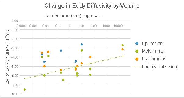
Figure 8 – The comparison of eddy diffusivity and the lake volume.

Figure 8 shows that the overall eddy diffusivity values for the metalimnion is lower, there is no strong correlation of the metalimnion eddy diffusivities with the logarithmic Pearson’s correlation of R² < 0.5.

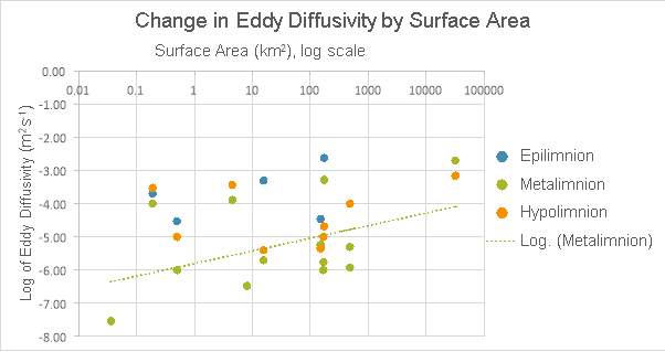
Figure 9 – The comparison of eddy diffusivity and the surface area of the lake.

Figure 9 shows a similar scatter plot to Figure 8, this shows the known correlation between the volume and surface area. The trendline here too shows that there is no significant correlation as R²< 0.5.

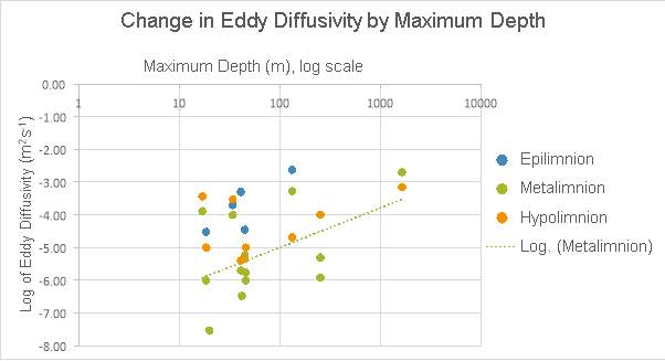
Figure 10 – The comparison of eddy diffusivity and the maximum depth of the lake.

Figure 10, shows the maximum depth varies from a range of around 15m to over 1000m. The Pearson’s correlation does not show a value of significance, R²< 0.5.

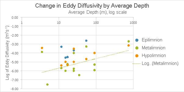
Figure 11 – The comparison of eddy diffusivity and the average depth of the lake.

Figure 11 clearly shows how the epilimnion values are higher than the other layers of eddy diffusivities. There is also a clear similarity between Figure 10 and Figure 11, showing that the average depth and maximum depth are linked, however the average depth does not have as a great a range.

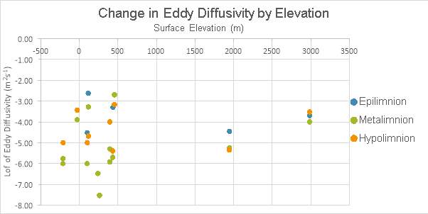
Figure 12 – The comparison of eddy diffusivity and the elevation of the lake.

Figure 12 shows very little obvious correlation. The Pearson’s correlation R² < 0.01. There are some negative elevation values which show that some of the lakes are below sea level, which is unusual.

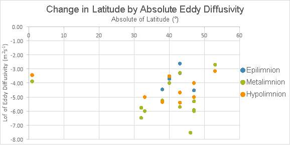
Figure 13 – The comparison of eddy diffusivity and the absolute latitude of the lake.

Figure 13 had a Pearson’s correlation R² < 0.01, showing no significant correlation. It is evident that the latitudes of lakes are similar, with only one being near the equator at absolute latitude between 0 and 10°.

8.2 PCA (Principle Component Analysis)

To interpret the data and determine whether a relationship between the eddy diffusivity values and the physical features of the lake can be drawn and what that relationship might be a Principle Component Analysis was conducted. The results are in table XX.

To assess the significance of the PCA results, a Bartletts test for Sphericity was carried out. It passed, the Critical Chi-squared value was 29.6 and the observed Chi-squared value was 211.5. This shows that there is correlation in the data.

The Principle Component Analysis compares multiple variables at once and looks to see if there are correlated. Factor F1 represents the first principle component, it is the linear combination of variables that have the maximum variance. The second principle component must have 0 correlation with Principle component 1 and accounts for second greatest variation. All subsequent principle components are linear combinations that have no correlation with existing principle components.

Table 2 shows how much each principle component (F) value attributes to the variability of the data. As you can see the first three components (F1, F2 and F3) contribute over 95% of the variance, so F4, F5, F6 and F7 can be regarded as negligible.

Table 2 – Eigenvalue table showing the variability attributed to each principle component

	F1	F2	F3	F4	F5	F6	F7
Eigenvalue	4.470	1.121	1.075	0.315	0.017	0.001	0.000
Variability (%)	63.862	16.017	15.357	4.506	0.247	0.010	0.000
Cumulative %	63.862	79.879	95.236	99.742	99.989	100.000	100.000

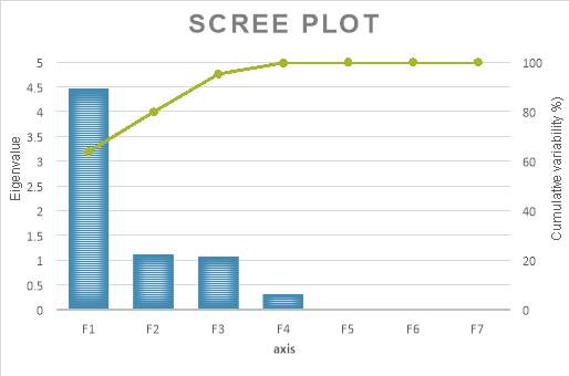
Figure 14 – Scree Plot of PCA analysis, showing the percentage of variance attributed to each principle component analysis and the associated eigenvalue

Figure 14, shows that if we consider the 95% variability, it only involves the first three principle components, F1, F2 and F3.

Table 3 shows the correlation between the variables and the principle component factors. A correlation> 0.5 has been highlighted to show the key relationships. Principle component 1 shows a very strong relationship between the lake size, having a score of 0.9 in the variables volume, surface area, maximum depth and average depth. This is as expected as the volume is directly linked to the surface area and the depth of the lake. Eddy Diffusivity is also positively linked to these variables. This shows that there is positive correlation between the eddy diffusivity and the size of the lake, the greater the size of the lake, the greater the eddy diffusivity. The second influencing factor shows a relationship between the eddy diffusivity and the elevation.

Table 3 – Contribution of variables to each significant Principle Component

	F1	F2	F3
Var1 = Vertical eddy diffusivity	0.621	0.573	-0.361
Var2 = Volume	0.987	-0.041	-0.040
Var3 = Surface Area	0.989	-0.044	-0.036
Var4 = Maximum Depth	0.993	-0.073	-0.003
Var5 = Average Depth	0.995	-0.064	-0.009
Var6 = Elevation	-0.042	0.846	0.490
Var7 = Latitude	0.396	-0.253	0.838

As shown in Figure 15 below as variables 2-5 are far from the centre and very close to one another, this means they are highly correlated. Variable 6 is almost perpendicular to these variables which means that they are not correlated.
Variable 1, shows a degree of correlation to the size profile and the elevation, this shows that it can be influenced by both the size of the lake and the elevation.

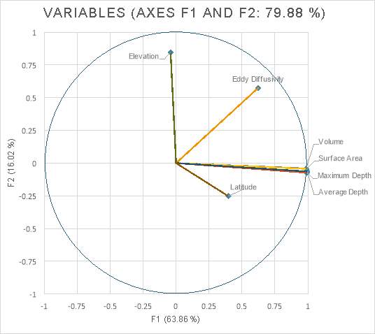
Figure 15 – Correlation Circle, showing how the variables are linked with the first two principle components

Figure VV

9.0 Discussion

9.1 Table of results

The results table, Table AA shows that epilimnion has the greatest eddy diffusivity value, this is to be expected as the driving force for mixing, wind, occurs here and the subsequent energy is transferred through the layers and some can be expected to have been dissipated down the depth. Weak winds will cause turbulence in the boundary layer of the epilimnion, that is not substantial enough to cause internal waves, this causes an increase in the eddy diffusivity value for the epilimnion.

Table AA showed a lower eddy diffusivity value for the metalimnion than the hypolimnion and epilimnion, this means that less mixing takes place near the thermocline. This is as expected, from the diagram (insert ref to picture in lit review), you can see that the mixing near the thermocline is reduced.

9.2 Discrepancy in eddy diffusivity values

Looking more closely at the values in Table AA for the lakes that have two data sets, a discrepancy is evident. A difference of: Mono Lake = 1.17 x 10^-6, Lake Constance = 3.8 x 10^-6 and Lake Kinneret = 7.34 x 10^-7. Putting that into perspective the percentage difference is: Mono Lake 20.4 %, Lake Constance 76.1 %, Lake Kinneret 73.44 %.

The molecular diffusion for heat in water, K_M, is 1.5 x 10^-7. In Table AA, the metalimnion value for the eddy diffusivity in Crystal Lake is below this, at 2.93 x 10^-8. Theoretically, the eddy diffusivity value should never be below the molecular diffusion of heat in water, as eddy diffusion can only enhance the rate of mixing and not reduce it. This value is likely to be inaccurate, with an average depth of only 4.9m, there is potential that this lake is too shallow to have significant stratification. As shown in the method section, this data set was one of them that had been derived from the lake number following the research by (Yeates & Imberger, 2003), the crystal lake has particularly high lake number. An error in the assumption here could be the cause.

Lake	Eddy Diffusivity Data (m2s-1)
	Epilimnion	Metalimnion	Hypolimnion
Mono Lake (1)	3.50E-05	5.75E-06	4.50E-06
Mono Lake (2)		4.58E-06
Lake Constance (1)	1.00E-04	5.00E-06	1.00E-04
Lake Constance (2)		1.20E-06
Lake Kinneret (1)	1.00E-05	1.00E-06	1.00E-05
Lake Kinneret (2)		1.73E-06

There is a cluster of lakes studied in the northern temperate zone, this is likely to be because this is part of the developed world where they have the luxury of research so there is more data available. Also, most of the locations are from areas which are English speaking: Australia and the USA making up over half the lakes 7 out of 11, this may be because this research was limited to papers written in English and there could be further research that is reported in other languages that has not been considered.

9.3 PCA

The combination of Table 2 and Table 3, show that the first principle component, which accounts for the most variance is related to the lake properties and the eddy diffusivity value. This means that the strongest correlation can be seen between these. The data in the PCA may have been skewed, because there are several properties that are related to the “size” of the lake. It may have been better to use one size ratio that combines the profile properties and use that. The strong correlation indicates that there is a relationship between the size of the lake and the eddy diffusivity. It states that the larger the lake, the larger the eddy diffusivity. This is as expected, as the greater the surface area of the lake, the greater energy is gathered from wind, which is transferred into energy in internal waves which causes the eddy diffusion at the metalimnion.

The second influencing factor, F2, is linked to the elevation and the eddy diffusivity, showing a positive correlation. This shows that the greater elevation has greater elevation, this is likely to be because greater elevation has greater wind speeds. There is also no shown correlation between the elevation and size of the lake, as demonstrated in both Table 3 and Figure 15. This shows evidence for what we already know, that lakes can vary size independently of elevation. The correlation shown between the latitude and size profile in Figure 15, due to being close together is probably a quirk, due to the small data set we are using.

Though the reliability of the results may be questioned considering only data on 11 lakes was found. A PCA is more reliable with a higher amount of data, as the number of data sets, 14, was close to the number of variables, 7, the PCA is likely to show a stronger correlation than what would be representative. Furthermore, PCA only considers linear trend, had there been a polynomial correlation, that would not have been spotted through a PCA. For this reason, the variables were also plotted against eddy diffusivity to look for any trend in the data.

10.0 Conclusion

This dissertation has explored the importance of protecting our freshwater sources and the risks they face, concluding that more research is necessary to better understand how lakes will be impacted with a decreased atmospheric content of oxygen and the expected rise in temperatures. This study includes information on the importance of mixing in seasonally stratified lakes and how a well-mixed lake helps maintain a healthy ecosystem.

Through analysing 11 lakes with 14 data sets a relationship between the eddy diffusivity coefficient and the properties of the lake has been established. Results showed that larger lakes have higher eddy diffusivities and the high the elevation the greater the eddy diffusivity. This means if a lake were to decrease in volume a lower rate of mixing may be expected. The analysis has demonstrated a correlation in rate of mixing in lakes across the world.

Future research into the rate of vertical mixing in a wider range of lakes across the world is recommended, currently there is a concentration of lakes studied in the northern temperate regions, more research is necessary to establish the effect of climate change in equatorial and tropical regions.

Regional considerations of the impacts of climate change must be considered, especially any change to the nutrient supply of the lake. Though a global rise in temperature may expected, the change in different locations may vary considerably. For example, there is likely to be a shift in the wind patterns, causing some locations wind energy to increase, this would increase the rate of mixing and may alleviate the impact of longer stratification periods. Oher impacts of climate change, for example the nutrient supply will have impacts on lake quality and this need to b consider in a holistic view.

This research can contribute to the wider picture of understanding vertical mixing. It is crucial for more research to be undergone to understand how climate change will impact vertical mixing in lakes, and in turn secure drinking water supplies for future generations.

Bibliography

Angler Web, 2017. Anglerweb.com. [Online]
Available at: http://www.anglerweb.com/fishing_spots/lake-ada-hayden
[Accessed 25 March 2017].

Antenucci, J. P., Imberger, J. & Saggio, A., 2000. Seasonal evolution of the basin-scale internal wave field in a large stratified lake. Limnology and Oceanography, 45(7), pp. 1621-1638.

Blumberg, A. F. & Toro, D. M. D., 1990. Effects of Climate Warming on Dissolved Oxygen Concerntrations in Lake Erie. Transactions of the Americans Fisheries Society, 119(2), pp. 210-223.

Boehrer, B., Ilmberger, J. & Münnich, K. O., 2000. Vertical structure of currents in western Lake Constance. Geophysical Research, 105(12), pp. 28823-28835.

Carr, J. F. & Hiltunen, J. K., 1965. CHANGES IN THE BOTTOM FAUNA OF WESTERN LAKE. Limnolgy and Oceanography, 10(4), pp. 551-569.

Coats, R. P.-L. J. S. G. e. a., 2006. The Warming of Lake Tahoe. Climatic Change, 76(1), pp. p121-148.

Department of Environmental Consideration, 2017. New York State: Cayuga Lake. [Online]
Available at: http://www.dec.ny.gov/outdoor/36544.html
[Accessed 25 March 2017].

Dorostkar, A. & Boegman, L., 2013. Internal hydraulic jumps in a long narrow lake. Limnology and Oceanography, 58(1), pp. 153-172.

European Commission, 2015. Horizon 2020: Turning sea water into drinking water. [Online]
Available at: https://ec.europa.eu/programmes/horizon2020/en/news/turning-sea-water-drinking-water
[Accessed 3 March 2017].

Fischer, H. B. et al., 1979. Mixing in Inland and Coastal Waters. London: Academic Press, Inc.

Foley, B., Jones, I. D., Maberley, S. C. & Rippey, B., 2011. Long-term changes in oxygen depletion in a small temperate. Freshwater Biology, 57(2), pp. 278-289.

Freemap tools, 2017. freemaptools: elevation finder. [Online]
Available at: https://www.freemaptools.com/elevation-finder.htm
[Accessed 25 March 2017].

Gautam, R. K., Sharma, S. K., Mahiya, S. & Chattopadhyaya, M. C., 2014. Contamination of Heavy Metals in Aqautic Media: Transport, Toxicity and Technologies for Remediation. In: S. K. Sharma, ed. Heavy Metals In Water: Presence, Removal and Safety. Cambridge: The Royal Society of Chemistry, pp. 1-18.

Geology.com, 2005. Geoscience News and Information: Deepst Lake in the World. [Online]
Available at: http://geology.com/records/deepest-lake.shtml
[Accessed 25 March 2017].

GLIN, n.d. Great Lakes. [Online]
Available at: http://www.great-lakes.net/teach/pollution/water/water5.html
[Accessed 15 December 2016].

Google Maps, 2017. Google Maps. [Online]
Available at: https://www.google.co.uk/maps?hl=en
[Accessed 3 April 2017].

Iowa Great Lakes Association, 2017. Iowa Great Lakes Association: Lake Maps, Sizes and Depths. [Online]
Available at: http://iagreatlakes.com/preserving-the-lakes/great-lakes-maps/
[Accessed 25 March 2017].

iowa.com, 2017. IOWA: Department of Natural Resources. [Online]
Available at: http://www.iowadnr.gov/Fishing/Where-to-Fish/Lakes-Ponds-Reservoirs/LakeDetails/lakeCode/AHL85
[Accessed 25 March 2017].

Israel Limnology and Oceanography Research, 2017. Israel Limnology and Oceanography Research: Lake Kinneret. [Online]
Available at: http://www.ocean.org.il/eng/kineret/lakekineret.asp
[Accessed 25 March 2017].

Jassby, A. & Powell, T., 1975. Vertical Patterns of eddy diffusivity during stratification in Castle Lake, California. Limnology and Oceanography, 20(4), pp. 530-543.

Jeppesen, E. et al., 2000. Trophic Structure, species richness and biodiversity in Danish lakes: changes over a phosphorus gradient. Freshwater Biology, 45(2), pp. 201-218.

Lakepedia.com, 2015. Lakepedia: Lake Constance. [Online]
Available at: https://www.lakepedia.com/lake/constance.html
[Accessed 25 March 2017].

Lars J. Tranvik, J. A. D. J. B. C. S. A. L. G. S., 2009. Lakes and reservoirs as regulators of carbon cycling and climate. Limnology and Oceanography, 54(6), p. 2298–2314.

Laval, B. E., Imberger, J. & Findikakis, A. N., 2005. Dynamics of a large tropical lake: Lake Maracaibo. Aquatic Sciences, Volume 67, pp. 337-349.

Live Science, 2017. Live Science: Lake Baikal. [Online]
Available at: http://www.livescience.com/57653-lake-baikal-facts.html
[Accessed 25 March 2017].

Livingsone, D. M., 2003. Impact of Secular Climate Change on the Thermal Structure of a Large Temperate Central European Lake. Climatic Change, pp. Volume 57, Issue 1, Pages 205-207.

Matear, R. J., Hirst, A. C. & McNeil, B. C., 2000. Changes in dissolved oxygen in the Southern Ocean with climate change. Geochemistry, Geophysics, Geosystems, 1(11).

McIntyre, S., Clark, J. F. & Jellison, R., 2009. Turbulent mixing induced by nonlinear internal waves in Mono Lake, California. American Society of Limnology and Oceanography, Inc, 54(6), pp. 2255-2271.

Mono Lake Committee, 2017. Mono Lake Committee: Quick Facts. [Online]
Available at: http://www.monolake.org/about/stats
[Accessed 25 March 2017].

Müller, B., Bryant, L. D., Matzinger, A. & Wüest, A., 2012. Hypolimnetic Oxygen Depletion in Eutrophic Lakes. Environmental Science and Technology, 46(18), p. 9964–9971.

National Geographic Partners LLC, 2016. National Geographic. [Online]
Available at: http://environment.nationalgeographic.com/environment/freshwater/freshwater-crisis/
[Accessed 15 December 2016].

Pannard, A. et al., 2011. Recurrent internal waves in a small lake: Potential ecological consequences for metalimnetic phytoplankton populations. Limnology and Oceanography: Fluids and Environments, 1(1), pp. 91-109.

Perlman, H., 2016. United States Geological Survey: Water Science School. [Online]
Available at: https://water.usgs.gov/edu/qa-home-percapita.html
[Accessed 8 March 2017].

Scripps O2 Programme, 2016. Scripps O2 Programme: Atmospheric Oxygen Research. [Online]
Available at: http://scrippso2.ucsd.edu/
[Accessed 3 March 2017].

The Columbia Encyclopedia, 2016. Encyclopedia.com. [Online]
Available at: http://www.encyclopedia.com/places/germany-scandinavia-and-central-europe/central-european-physical-geography/lake-constance
[Accessed 25 March 2017].

Wain, D. J., Kohn, M. S., Scanlon, J. A. & Rehmann, C. R., 2013. Internal wave-driven transport of fluid away from the boundary of a lake. Association for the Sciences of Limnology and Oceanography, 58(2), pp. 429-442.

Wain, D. J. & Rehmann, C. R., 2010. Transport by an intrusion generated by boundary mixing in a lake. Water Resources Research, Volume 46, p. W08517.

Wikipedia, 2017. Wikipedia: Castle Lake. [Online]
Available at: https://en.wikipedia.org/wiki/Castle_Lake_(California)
[Accessed 25 March 2017].

Wikipedia, 2017. Wikipedia: Crystal Lake. [Online]
Available at: https://en.wikipedia.org/wiki/Crystal_Lake_(Gilmanton,_New_Hampshire)
[Accessed 25 March 2017].

Wikipedia, 2017. Wikipedia: Kranji Reservoir. [Online]
Available at: https://en.wikipedia.org/wiki/Kranji_Reservoir
[Accessed 25 March 2017].

Wikipedia, 2017. Wikipedia: Lake Baikal. [Online]
Available at: https://en.wikipedia.org/wiki/Lake_Baikal
[Accessed 3 April 2017].

Williams, A. E., Waterfall, R. J., White, K. N. & Hendry, K., 2010. Manchester Ship Canal and Salford Quays: Industrial Legacy and Ecological Restoration. In: B. L., ed. Ecological Reviews: Ecology of Industrial Pollution. Manchester: Cambridge University Press, pp. 276-308.

World Lake Database, 2017. World Lake Database: Cayuga Lake. [Online]
Available at: http://wldb.ilec.or.jp/data/databook_html/nam/nam-17.html
[Accessed 25 March 2017].

Wüest, A. & Lorke, A., 2003. Small-Scale Hydrodynamics in Lakes. Fluid Mechanics, Volume 35, pp. 373-412.

Yang, P. et al., 2014. Observatoins of vertical eddy diffusivities in a shallow tropical reservoir. Hydro-environment Research, 9(3), pp. 441-451.

Yeates, P. S. & Imberger, J., 2003. Pseudo two-dimensional simulations of internal and boundary fluxes in stratified lakes and reservoirs. Internation Journal of River Basin Management, 1(4), pp. 297-319.

Appendix

Table 4 References correlating to the data found for the table of results

Lake	Eddy Diffusivity	Volume	Surface Area	Max Depth	Av Depth	Elevation	Latitude
Mono Lake (1)	(McIntyre, et al., 2009)	(Mono Lake Committee, 2017)	(McIntyre, et al., 2009)	(McIntyre, et al., 2009)	(Mono Lake Committee, 2017)	(Google Maps, 2017)	(Yeates & Imberger, 2003)
Lake Constance (1)	(Boehrer, et al., 2000)	(Boehrer, et al., 2000)	(The Columbia Encyclopedia, 2016)47	(The Columbia Encyclopedia, 2016)	(Lakepedia.com, 2015)	(Google Maps, 2017)	(Yeates & Imberger, 2003)
Castle Lake	(Jassby & Powell, 1975)	–	(Wikipedia, 2017)	(Wikipedia, 2017)	(Jassby & Powell, 1975)	(Google Maps, 2017)	(Google Maps, 2017)
Lake Ames	(Wain & Rehmann, 2010)	–	(iowa.com, 2017)	(iowa.com, 2017)	(Angler Web, 2017)	(Freemap tools, 2017)	(Google Maps, 2017)
West Okoboji Lake, Iowa	(Wain, et al., 2013)	–	(Iowa Great Lakes Association, 2017)	(Iowa Great Lakes Association, 2017)	(Iowa Great Lakes Association, 2017)	(Google Maps, 2017)	(Google Maps, 2017)
Lake Baikal	(Wüest & Lorke, 2003)	(Live Science, 2017)	(Live Science, 2017)	(Geology.com, 2005)	(Live Science, 2017)	(Wikipedia, 2017)	(Google Maps, 2017)
Kranji Reservoir	(Yang, et al., 2014)	(Wikipedia, 2017)	(Wikipedia, 2017)	(Wikipedia, 2017)	(Wikipedia, 2017)	(Freemap tools, 2017)	(Google Maps, 2017)
Cayuga Lake	(Dorostkar & Boegman, 2013)	(Department of Environmental Consideration, 2017)	(Dorostkar & Boegman, 2013)	(Department of Environmental Consideration, 2017)	(World Lake Database, 2017)	(Google Maps, 2017)	(Google Maps, 2017)
Lake Kinneret (1)	(Yeates & Imberger, 2003)	(Israel Limnology and Oceanography Research, 2017)	(Israel Limnology and Oceanography Research, 2017)	(Israel Limnology and Oceanography Research, 2017)	(Israel Limnology and Oceanography Research, 2017)	(Google Maps, 2017)	(Google Maps, 2017)
Lake Constance (2)	(Yeates & Imberger, 2003)	(Boehrer, et al., 2000)	(Yeates & Imberger, 2003)	(Yeates & Imberger, 2003)	(Lakepedia.com, 2015)	(Google Maps, 2017)	(Yeates & Imberger, 2003)
Mono Lake (2)	(Yeates & Imberger, 2003)	(Mono Lake Committee, 2017)	(McIntyre, et al., 2009)	(McIntyre, et al., 2009)	(Mono Lake Committee, 2017)	(Google Maps, 2017)	(Yeates & Imberger, 2003)
Lake Kinneret (2)	(Yeates & Imberger, 2003)	(Israel Limnology and Oceanography Research, 2017)	(Israel Limnology and Oceanography Research, 2017)	(Israel Limnology and Oceanography Research, 2017)	(Israel Limnology and Oceanography Research, 2017)	(Google Maps, 2017)	(Yeates & Imberger, 2003)
Crystal Lake	(Yeates & Imberger, 2003)	(Wikipedia, 2017)	(Yeates & Imberger, 2003)	(Yeates & Imberger, 2003)	(Wikipedia, 2017)	(Freemap tools, 2017)	(Yeates & Imberger, 2003)
Mundaring Reservoir	(Yeates & Imberger, 2003)	–	(Yeates & Imberger, 2003)	(Yeates & Imberger, 2003)	–	(Freemap tools, 2017)	(Yeates & Imberger, 2003)